The representer theorem of [40] provides an analytic form to the MAP solution for a large class of likelihoods within the kernel framework, and in Chapter 2 a similar representation for the posterior process in the Bayesian framework was provided. However, when making predictions, these parametrisations require all data. The aim of this chapter is to propose a solution in which the prediction is given in terms of a subset of the data, which will be referred to as the set of Basis Vectors and the solution as sparse solution.
Sparsity in non-parametric families is important since the typical data set size for real applications can be very large. Although theoretically attractive, due to their ``non-parametric nature'' the kernel methods are of restricted usage; they cannot be easily applied for extracting information from large datasets. This is illustrated for example by the quadratic scaling of the number of parameters with the size of the data set for the GP.
Predictions involving a small subset of the original data were given
originally for classification using the Support Vector Machines
(SVM) [93] and then extended to treat regression. These
results are batch solutions that require an optimisation with
respect to the full dataset. Usually there are efficient solutions
to the problem when the data is small, but these solutions are not
feasible for large datasets. In recent years iterative methods were
developed that break down the optimisation problem into subproblems
such as chunking [59], or the sequential minimal
optimisation [61]. These methods were developed to the SVMs
with an ![]() -insensitive loss function for the regression and
the classification case.
-insensitive loss function for the regression and
the classification case.
The sparse representation in SVMs is a result of the
non-differentiable nature of the cost functions, if we replace it for
example with a quadratic loss function, the solution is not sparse any
more. In this chapter we develop sparse solutions to arbitrary
likelihoods in the Bayesian GP framework. To do this, we first
consider the image
![]() (x) of an input
x in the feature space
(x) of an input
x in the feature space
![]()
![]() . The projection of all data points into
. The projection of all data points into
![]()
![]() defines a data-manifold with a usually much smaller dimension than the
dimension of the embedding space
defines a data-manifold with a usually much smaller dimension than the
dimension of the embedding space
![]()
![]() . Nevertheless, since the data is
more dispersed across the dimensions than in the input space, the
feature space projection gives more freedom for the linear algorithms
to find a solution for the regression or classification case. This
can be seen clearly when we perform linear regression in a feature
space corresponding to an infinite-dimensional RBF kernel: we have an
exact fit for arbitrary large data. Here we exploit the assumption
that the data-manifold is of a much lower dimensionality than the data
itself.1
. Nevertheless, since the data is
more dispersed across the dimensions than in the input space, the
feature space projection gives more freedom for the linear algorithms
to find a solution for the regression or classification case. This
can be seen clearly when we perform linear regression in a feature
space corresponding to an infinite-dimensional RBF kernel: we have an
exact fit for arbitrary large data. Here we exploit the assumption
that the data-manifold is of a much lower dimensionality than the data
itself.1
A first constraint to the problem was the prior on the parameters or the prior GP in the Bayesian framework from Chapter 2. Here the Bayesian solution will further constrained: we impose the resulting GP to be expressed solely based on a small subset of the data, using the parametrisation given in eq. (33).
The small subset is selected by sequentially building up the set of
basis points for the GP representation. This set, which is of a fixed
size, is called the set of ``basis vectors'' or
![]() set, is
introduced in the next section. This section also details previous
attempts and an intuitive picture for the sparse approximation. We
address the question of removing a basis vector that is already in the
GP by computing the KL-distance between two GPs in
Section 3.2. The KL-distance is computed using the
equivalence of the GPs with the normal distribution in the feature
space induced by the kernel.
set, is
introduced in the next section. This section also details previous
attempts and an intuitive picture for the sparse approximation. We
address the question of removing a basis vector that is already in the
GP by computing the KL-distance between two GPs in
Section 3.2. The KL-distance is computed using the
equivalence of the GPs with the normal distribution in the feature
space induced by the kernel.
The KL-distance is then used in a constrained optimisation framework
to find a process
![]() that is the closest possible to the
original one but has zero coefficients whenever the last
that is the closest possible to the
original one but has zero coefficients whenever the last
![]() is
encountered. The GP solution is independent of the order of the
is
encountered. The GP solution is independent of the order of the
![]() ,
meaning that any of the inputs can be put in the last position.
We thus implement pivoting in the GP family parametrised in a
data-dependent coordinate system.
,
meaning that any of the inputs can be put in the last position.
We thus implement pivoting in the GP family parametrised in a
data-dependent coordinate system.
Sparsity using the KL-divergence and a constrained optimisation is presented in Section 3.3 with an estimation of the error in Section 3.4.
A combination of the online GP updates from the previous chapter and the constrained optimisation results in the sparse online updates (Section 3.5). The theory is coalesced into a sparse online algorithm in Section 3.6. The subject of efficient low-dimensional representations in the framework of the non-parametric kernel method is under an intense study and we give an overview of the different approaches to sparsity in Section 3.7. We conclude the chapter with discussions and a list of possible future research directions.
We start the discussion about sparsity by having a closer look at the
online learning algorithm introduced in Chapter 2. The
algorithm adds a single input to the GP at each step, this addition
implies the extension of the basis in which we expressed the GP, given
in eq. (33). If the new input was in the linear span of
all previous inputs, then the addition of a new vector in the basis is
not necessary. Indeed, if we write
![]() as
as
and we substitute it in the update eq. (54) for the last feature vector, then an equivalent representation of the GP can be made that uses only the first t feature vectors. Unfortunately eq. (60) does not hold for most of the cases. Again, using as an example the popular RBF kernels, any set of distinct points maps to a linearly independent set of feature vectors. The feature space is a linear Hilbert space, and we use the linear algebra to decompose the new feature vector into (1) a component that is included in the subspace of the first t features and (2) one that is orthogonal to it and write
where the first term is the orthogonal projection expressed in a
vectorial form with the coordinates of the projection
![]() = [
= [![]() (1),...,
(1),...,![]() (t)]T. All previous feature
vectors have been grouped into the vector
(t)]T. All previous feature
vectors have been grouped into the vector
![]() t = [
t = [![]() ,...,
,...,![]() ] and
] and
![]() is the residual, the unit
vector orthogonal to the first t feature vectors. The squared
length of the residual is
is the residual, the unit
vector orthogonal to the first t feature vectors. The squared
length of the residual is
![]() = |
= |![]() -
- ![]() |2 with the norm in the
feature space given by
|2 with the norm in the
feature space given by
![]() a,a
a,a![]() = |a|2; the scalar
product is defined using the kernel
= |a|2; the scalar
product is defined using the kernel
![]()
![]() ,
,![]()
![]() = K0(x,y) and
= K0(x,y) and
![]() denotes
the approximation to
denotes
the approximation to
![]() in the subspace of all previous
inputs. The squared length of the residual
in the subspace of all previous
inputs. The squared length of the residual
![]() > 0 appears
also in the recursive computation of the determinant of the kernel
Gram matrix:
> 0 appears
also in the recursive computation of the determinant of the kernel
Gram matrix:
![]() Kt + 1
Kt + 1![]() =
= ![]() Kt
Kt![]()
![]() (see Appendix C or [43] for
details). If we proceed sequentially, then a way of keeping the kernel
matrix nonsingular is to avoid the inclusion of those elements for
which
(see Appendix C or [43] for
details). If we proceed sequentially, then a way of keeping the kernel
matrix nonsingular is to avoid the inclusion of those elements for
which
![]() = 0. This is a direct consequence of the linearity of
the feature space and in applications helps to keep the algorithm
stable, will avoid singular or almost singular kernel Gram matrices.
= 0. This is a direct consequence of the linearity of
the feature space and in applications helps to keep the algorithm
stable, will avoid singular or almost singular kernel Gram matrices.
Fig. 3.1 provides a visualisation of the inputs and
the projection in the feature space. We plotted the residual vector
![]() that is orthogonal to the span of the previous feature
vectors with squared length
that is orthogonal to the span of the previous feature
vectors with squared length
![]() .
.
![\includegraphics[]{project.eps}](img289.png)
|
An intuitive modification of the online algorithm is to project the
feature space representation of the new input when the error caused by
this projection is not too large. As a heuristic we can define the
errors as being the length of the residual
![]() . We might
justify this choice by the assumption that the inputs are not random,
i.e. they lie on a lower-dimensional manifold in the feature space.
The geometric consideration from Fig. 3.1 builds a
linear subspace onto which the inputs are projected using
eq. (61). This subspace however does not consider the
noise on the outputs, thus might be suboptimal, i.e. include into the
representation inputs that are coming from a noisy region of the data,
wasting resources.
. We might
justify this choice by the assumption that the inputs are not random,
i.e. they lie on a lower-dimensional manifold in the feature space.
The geometric consideration from Fig. 3.1 builds a
linear subspace onto which the inputs are projected using
eq. (61). This subspace however does not consider the
noise on the outputs, thus might be suboptimal, i.e. include into the
representation inputs that are coming from a noisy region of the data,
wasting resources.
To implement this sparse algorithm, we need to compute the projection
coordinates
![]() and the squared distance
and the squared distance
![]() from eq. (61). These values are obtained from minimising
the squared distance
|
from eq. (61). These values are obtained from minimising
the squared distance
|![]() -
- ![]() |2. Expanding
|2. Expanding
![]() using eq. (61) and replacing the
scalar products in the feature space with the corresponding kernel
functions, we have the following equation to minimise:
using eq. (61) and replacing the
scalar products in the feature space with the corresponding kernel
functions, we have the following equation to minimise:
where
Kt is the kernel matrix and
kt + 1 = [K0(x1,xt + 1),..., K0(xt,xt + 1)]T and
k* = K0(xt + 1,xt + 1), kernel functions obtained using
K0(xi,xj) = ![]()
![]() ,
,![]()
![]() . The differentiating it with
respect to the unknowns
. The differentiating it with
respect to the unknowns
![]() we obtain a linear system
with solution
we obtain a linear system
with solution
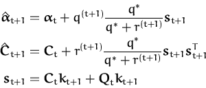
The changes in the online updates from Chapter 2 as a
result of this projection are minimal: the new parameters
(![]() t + 1,Ct + 1) are computed using
t + 1,Ct + 1) are computed using
instead of
st + 1 in eq. (57), thus the projected
parameters replace the true inputs. The result of this substitution
is important: although the new example has been processed, the
size of the model parameters is not increased. The computation
of
![]() however requires the inverse of the Gram matrix,
a costly operation. The following formula gives an online update to
the inverse Gram matrix
Qt + 1 = Kt + 1-1 which is based on
the matrix inversion lemma (see Appendix C for details):
however requires the inverse of the Gram matrix,
a costly operation. The following formula gives an online update to
the inverse Gram matrix
Qt + 1 = Kt + 1-1 which is based on
the matrix inversion lemma (see Appendix C for details):
where
et + 1 is the t + 1-th unit vector and
![]() = Qtkt + 1 is the projection from
eq. (62). The length of the residual is also
expressed recursively:
= Qtkt + 1 is the projection from
eq. (62). The length of the residual is also
expressed recursively:
![]() = k* - kt + 1TQtkt + 1 = k* - kt + 1T
= k* - kt + 1TQtkt + 1 = k* - kt + 1T![]() .
.
Observe that, in order to match the dimensions of the elements, we
have to add an empty last row and column to
Qt and a zero last
element to
![]() before performing the update. The
addition of the zero element can formally be written using functions
that do this operation. This simpler form of writing the equations
without the extra function for some components has been chosen to
preserve clarity.
before performing the update. The
addition of the zero element can formally be written using functions
that do this operation. This simpler form of writing the equations
without the extra function for some components has been chosen to
preserve clarity.
The idea of projecting the inputs to a linear subspace specified by a subset has been proposed by [95, Chapter 7] (or more recently by [96] and [73]) using a batch framework and maximum a-posteriori solutions.
Writing the MAP solutions as a linear combination of the input
features
![]() =
= ![]()
![]()
![]() , the projection to
the subset is obtained using the approximation
, the projection to
the subset is obtained using the approximation
![]()
![]()
![]()
![]() (j)
(j)![]() for each
input,
{
for each
input,
{![]() }j = 1, k being the subset onto which the inputs are
projected.
}j = 1, k being the subset onto which the inputs are
projected.
If we perform the iterative computation of the inverse kernel matrix
from eq. (64) together with the GP update rules, we can
modify the online learning rules in the following manner: we keep only
those inputs whose squared distance from the linear subspace spanned
by the previous elements is higher then a predefined positive
threshold
![]() >
> ![]() . This way we arrive at a sparse online GP algorithm. This modification of the online
learning algorithm for the GP family has been proposed by us
in [19,18]. Performing this modified GP
update sequentially for a dataset, there will be some vectors for
which the projection is used and others that will be kept by the GP
algorithm. In the following we will call the set of inputs the set of Basis Vectors for the GP and we will use the notation
. This way we arrive at a sparse online GP algorithm. This modification of the online
learning algorithm for the GP family has been proposed by us
in [19,18]. Performing this modified GP
update sequentially for a dataset, there will be some vectors for
which the projection is used and others that will be kept by the GP
algorithm. In the following we will call the set of inputs the set of Basis Vectors for the GP and we will use the notation
![]() for an element of the set and
for an element of the set and
![]() set for the whole set Basis Vectors.
set for the whole set Basis Vectors.
The online algorithm sketched above is based on ``measuring'' the
novelty in the new example with respect to the set of all previous
data. It may or may not add the new input to the
![]() set. on the
other hand, there might be cases when there is a new input which is
regarded ``important'' but due to the limitations of the machines we
cannot include it into the
set. on the
other hand, there might be cases when there is a new input which is
regarded ``important'' but due to the limitations of the machines we
cannot include it into the
![]() set. There might not be enough
resources available, thus it would be necessary to remove an existent
set. There might not be enough
resources available, thus it would be necessary to remove an existent
![]() to allow the inclusion of the new data.
to allow the inclusion of the new data.
However by looking at the new data only, there are no obvious ways to
remove an element from the
![]() set. A heuristic was proposed
in [19] by assuming that the GP is approximately
independent of the order of the presentation of the data. This
independence lead to the permutability of the order of presentation
and thus when removing a
set. A heuristic was proposed
in [19] by assuming that the GP is approximately
independent of the order of the presentation of the data. This
independence lead to the permutability of the order of presentation
and thus when removing a
![]() element we assumed that it was the last
added to the
element we assumed that it was the last
added to the
![]() set. The approximation of the feature vector
set. The approximation of the feature vector
![]() with its projection
with its projection
![]() from
eq. (61) was made, effectively removing the input
from
eq. (61) was made, effectively removing the input
![]() from the
from the
![]() set. The error due to the approximation
has also been estimated by measuring the change in the mean function
of the GP due to the substitution. The change was measured at the
inputs present in the
set. The error due to the approximation
has also been estimated by measuring the change in the mean function
of the GP due to the substitution. The change was measured at the
inputs present in the
![]() set and the location of the new example.
Since the projection into the subspace spanned by the previous data
was orthogonal, the mean function of the GP was changed only at the
new input with the change induced being
set and the location of the new example.
Since the projection into the subspace spanned by the previous data
was orthogonal, the mean function of the GP was changed only at the
new input with the change induced being
where the substitution
Qt + 1(t + 1, t + 1) = ![]() is based
on the iterative inversion of the inverse Gram matrix from
eq. (64). The score
is based
on the iterative inversion of the inverse Gram matrix from
eq. (64). The score
![]() can be computed not
only for the last element, but, by assuming permutability of the GP
parameters, for all elements in the
can be computed not
only for the last element, but, by assuming permutability of the GP
parameters, for all elements in the
![]() set. Its computation is
simple if we have the inverse Gram matrix and in the online algorithm
this was the criterion for removing an element from the
set. Its computation is
simple if we have the inverse Gram matrix and in the online algorithm
this was the criterion for removing an element from the
![]() set. This
score is lacking the probabilistic characteristic of the Gaussian
processes in the sense that in computing it we ignore the changes in
the kernel functions.
set. This
score is lacking the probabilistic characteristic of the Gaussian
processes in the sense that in computing it we ignore the changes in
the kernel functions.
Later in this chapter the heuristics discussed so far is replaced with a different approach to obtain sparsity: we compute the KL-divergence between the Gaussian posterior and a new GP that is constrained to have zero coefficients corresponding to one of the inputs. That input is then removed from the GP.
We are mentioning that removing the last element is a choice to keep
the computations clear, all the previously mentioned operations are
extended in a straightforward manner to any of the basis vectors in
the
![]() set by permuting the order of the parameters.
Section 3.2 presents the basis of the sparse online
algorithms: the analytic expression of the KL-divergence in the GP
family.
set by permuting the order of the parameters.
Section 3.2 presents the basis of the sparse online
algorithms: the analytic expression of the KL-divergence in the GP
family.
In online learning we are building approximations based on minimising a KL-divergence. The learning algorithm from Chapter 2 was based on minimising the KL-distance between an analytically intractable posterior and a simple, tractable one. The distance measures thus play an important role in designing approximating algorithms. Noting the similarity between the GP and the finite-dimensional normal distributions, we are interested in obtaining some distance measures in the family of Gaussian processes.
In this section we will compute the ``distance'' between two GPs based
on the representation lemma in Chapter 2 (also
[19]) using the observation that GPs can be viewed
as normal distributions with the mean
![]() and the covariance
and the covariance
![]() given as functions of the input data, shown in
eq. (47).
given as functions of the input data, shown in
eq. (47).
If we consider two GPs using their feature space notation, then we have an analytical form for the KL-divergence [41] by integrating out eq. (26):
where the means and the covariances are expressed in the
high-dimensional and unknown feature space. The trace term on the RHS
includes the identity matrix in the feature space, this was obtained
by the substitution
![]() where
where
![]() is the
``dimension'' of the feature space. We will express this measure in
terms of the GP parameters and the kernel matrix at the basis points.
is the
``dimension'' of the feature space. We will express this measure in
terms of the GP parameters and the kernel matrix at the basis points.
The two GPs might have different
![]() sets. Without loosing generality,
we unite the two
sets. Without loosing generality,
we unite the two
![]() sets and express each GP using this union by
adding zeroes to the inputs that were not present in the respective
set. Therefore in the following we assume the same support set for both
processes. The means and covariances are parametrised as in
eq. (47) with
(
sets and express each GP using this union by
adding zeroes to the inputs that were not present in the respective
set. Therefore in the following we assume the same support set for both
processes. The means and covariances are parametrised as in
eq. (47) with
(![]() 1,C1) and
(
1,C1) and
(![]() 2,C2) and the corresponding elements have the same
dimensions.
2,C2) and the corresponding elements have the same
dimensions.
We will use the expressions for the mean and the covariance functions
in the feature space:
![]() =
= ![]()
![]() and
and
![]() from eq. (48) with
from eq. (48) with
![]() =
= ![]() B the concatenation of all
B the concatenation of all
![]() elements expressed in the
feature space. The KL-divergence is transformed so that it will
involve only the GP parameters and the inner product kernel matrix
KB =
elements expressed in the
feature space. The KL-divergence is transformed so that it will
involve only the GP parameters and the inner product kernel matrix
KB = ![]() T
T![]() . This eliminates the matrix
. This eliminates the matrix
![]() in which the
number of columns equals the dimension of the feature space. For this
we transform the inverse covariance using the matrix inversion lemma
as
in which the
number of columns equals the dimension of the feature space. For this
we transform the inverse covariance using the matrix inversion lemma
as
and using this result we obtain the term involving the means as
where we assumed that the kernel matrix including all data points
KB is invertible. The matrix inversion lemma
eq. (181) has been used in the opposite direction to
obtain eq. (69). The condition of
KB being invertible
is not restrictive since a singular kernel matrix implies we can find
an alternative representation of the process that involves a
non-singular kernel matrix (i.e. linearly independent basis points,
see the observation at eq. (61)). For the second term of
eq. (66) we use the property of traces
![]() . Using eq. (67) again we obtain
. Using eq. (67) again we obtain
This provides a representation of the trace using the kernel matrix and the parameters of the two GPs. For the third term in eq. (66) we are using the property of the log-determinant
together with the permutability of the components in traces and
obtain
In deriving the smaller dimensional representation from eq. (72) the permutability of the matrices inside the trace function has been used as in eq. (70). This leads to the equation for the KL-distance between two GPs
![\includegraphics[]{bothKL.eps}](img333.png)
|
We see that the first term in the KL-divergence is the distance
between the means using the metric provided by
![]() . Setting
C2 = 0 we would have the matrix
KB as metric matrix for the
parameters of the mean. This problem was solved for the zero mean
functions and a diagonal restriction for
C1, the posterior
kernel, to obtain the ``Sparse kernel PCA'' [88],
discussed in details in Section 3.7.1.
. Setting
C2 = 0 we would have the matrix
KB as metric matrix for the
parameters of the mean. This problem was solved for the zero mean
functions and a diagonal restriction for
C1, the posterior
kernel, to obtain the ``Sparse kernel PCA'' [88],
discussed in details in Section 3.7.1.
We stress that the computation of the KL-distance is based on the parameters of the two GPs and the kernel matrix. It is important that the GPs share the same prior kernels so that the same feature space is used when expressing the means and covariances in eq. (48) for the Gaussians in the feature space.
As an example, let us consider the GPs at times t and t + 1 from the online learning scheme and compute the KL-divergences between them. Since the updates are sequential and include a single term each step, we expect that the KL-divergence between the old and new GP to be expressible using scalars. This is indeed the case as we can write the two KL-divergences in terms of scalar quantities:
where the parameters are taken from the online update rule
eq. (57) and
![]() = k* + kt + 1TCtkt + 1 is the variance of the
marginalisation of
= k* + kt + 1TCtkt + 1 is the variance of the
marginalisation of
![]() at
xt + 1. We plotted the evolution
of the pair of KL-divergences in Fig. 3.2 for a toy
regression example, the Friedman dataset #1 [23]. The
inputs are 10-dimensional and sampled independently from a uniform
distribution in [0, 1]. The output uses only the first 5
components
f (x) = sin(
at
xt + 1. We plotted the evolution
of the pair of KL-divergences in Fig. 3.2 for a toy
regression example, the Friedman dataset #1 [23]. The
inputs are 10-dimensional and sampled independently from a uniform
distribution in [0, 1]. The output uses only the first 5
components
f (x) = sin(![]() x1)x2 + 20(x3 - 0.5)2 + 10x4 + 5x5 +
x1)x2 + 20(x3 - 0.5)2 + 10x4 + 5x5 + ![]() with the last component a zero-mean unit variance random noise. The
noise variance in the likelihood model was
with the last component a zero-mean unit variance random noise. The
noise variance in the likelihood model was
![]() = 0.02. We see
that in the beginning the two KL-divergences are different, but as
more data are included in the GP, their difference gets smaller. This
suggests that the two distances coincide if we are converging to the
``correct model'', i.e. the Bayesian posterior. It can be checked
that the dominating factor in both divergences is
= 0.02. We see
that in the beginning the two KL-divergences are different, but as
more data are included in the GP, their difference gets smaller. This
suggests that the two distances coincide if we are converging to the
``correct model'', i.e. the Bayesian posterior. It can be checked
that the dominating factor in both divergences is
![]() ,
this factor will be of second order (i.e. of the fourth power of
,
this factor will be of second order (i.e. of the fourth power of
![]() ) if we subtract the two divergences (and expand the
logarithm up to the second order). Furthermore, since we are in the
Bayesian framework, the predictive variance
) if we subtract the two divergences (and expand the
logarithm up to the second order). Furthermore, since we are in the
Bayesian framework, the predictive variance
![]() tends to
zero as the learning progresses, thus we have that the two
KL-divergences converge.
tends to
zero as the learning progresses, thus we have that the two
KL-divergences converge.
It would be an interesting question to identify the exact differences between the two KL-divergences and try to interpret the distances accordingly. A straightforward exploration would be to relate the KL-divergence to the Fisher information matrix [43,14], which is well studied for the case of multivariate Gaussians2, hopefully a future research direction toward refining the online learning algorithm (see Section. 3.8.1).
Fixing the process
![]() , and imposing a constrained form to
, and imposing a constrained form to
![]() will lead to the sparsity in the family of GPs, presented next.
will lead to the sparsity in the family of GPs, presented next.
We next introduce sparsity by assuming that the GP is a result of some
arbitrary learning algorithm, not necessarily online learning. This
implies that at time t + 1 we have a set of basis vectors for the GP
and the parameters
![]() t + 1 and
Ct + 1. For simplicity we
will also assume that there are t + 1 elements in the
t + 1 and
Ct + 1. For simplicity we
will also assume that there are t + 1 elements in the
![]() set (its
size is not important). We are looking for the ``closest'' GP with
parameters
(
set (its
size is not important). We are looking for the ``closest'' GP with
parameters
(![]() ,
,![]() ) and with a reduced
) and with a reduced
![]() set where the last element
xt + 1 has been removed. Removing
the last
set where the last element
xt + 1 has been removed. Removing
the last
![]() means imposing the constraints
means imposing the constraints
![]() (t + 1) = 0 for the parameters of the mean and
(t + 1) = 0 for the parameters of the mean and
![]() (t + 1, j) = 0 for all
j = 1,..., N for the kernel. Due
to symmetry, the constraints imposed on the last column involve the
zeroing of the last row, thus the feature vector
(t + 1, j) = 0 for all
j = 1,..., N for the kernel. Due
to symmetry, the constraints imposed on the last column involve the
zeroing of the last row, thus the feature vector
![]() will not
be used in the representation.
will not
be used in the representation.
We solve a constrained optimisation problem, where the function to optimise is the KL-divergence between the original and the constrained GP (74):
The choice for the KL-divergence here is a pragmatic one: using the
KL-measure and differentiating with respect to the parameters of
![]() , we want to obtain an analytically tractable model.
Using
, we want to obtain an analytically tractable model.
Using
![]() does not lead to a simple
solution.
does not lead to a simple
solution.
In the following we will use the notation
Q = K-1 for the
inverse Gram matrix. Differentiating eq. (76) with
respect to all nonzero values
![]() ,
i = 1,..., t and
writing the resulting equations in a vectorial form leads to
,
i = 1,..., t and
writing the resulting equations in a vectorial form leads to
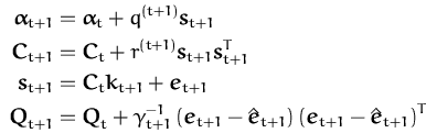
where It is the identity matrix and 0t is the column vector of length t with zero elements and [It0t] denotes a projection that keeps only the first t rows of the t + 1-dimensional vector to which it is applied. Solving eq. (77) leads to updates for the mean parameters as
where the elements of the updates are shown in Fig 3.3.
Differentiation with respect to the matrix
![]() leads to
the equation
leads to
the equation
where
![]() has only t rows and columns and the matrix
[It0t] used twice trims the matrix to the first t rows
and columns. The result is again expressed as a function of the
decomposed parameters from Fig 3.3 as
has only t rows and columns and the matrix
[It0t] used twice trims the matrix to the first t rows
and columns. The result is again expressed as a function of the
decomposed parameters from Fig 3.3 as
A reduction of the kernel Gram matrix is also possible using the quantities from Fig 3.3:
This follows immediately from the analysis of the iterative update of the inverse kernel Gram matrix Qt + 1 in eq. (64). The deductions use the matrix inversion lemma eq. (182) for Qt + 1 = Kt + 1-1 and (C + Q)-1, the details are deferred to Appendix D.
An important observation regarding the updates for the mean and the
covariance parameters is that we can remove any of the elements of the
set by permuting the order of the
![]() set and then removing the last
element from the
set and then removing the last
element from the
![]() set. For this we only need to read off the
scalar, vector, and matrix quantities from the GP parameters.
set. For this we only need to read off the
scalar, vector, and matrix quantities from the GP parameters.
Notice also the benefit of adding the inverse Gram matrix as a
``parameter'' and updating it when adding (eq. 64) or
removing (eq. 81) an input from the
![]() set: the updates
have a simpler form and the computation of scores is computationally
cheap. The propagation of the inverse kernel Gram matrix makes the
computations less expensive; there is no need to perform matrix
inversions. In experiments one could also use instead of the inverse
Gram matrix
Q its Cholesky decomposition, discussed in
Appendix C.2. This reduces the size of the algorithm
and keeps the inverse Gram matrix positive definite.
set: the updates
have a simpler form and the computation of scores is computationally
cheap. The propagation of the inverse kernel Gram matrix makes the
computations less expensive; there is no need to perform matrix
inversions. In experiments one could also use instead of the inverse
Gram matrix
Q its Cholesky decomposition, discussed in
Appendix C.2. This reduces the size of the algorithm
and keeps the inverse Gram matrix positive definite.
Being able to remove any of the basis vectors, independently of the order or the particular training algorithm used, the next logical step is to measure the effect of the removal, as presented next.
A natural choice for measuring the error is the KL-distance between
the two GPs,
![]() and
and
![]() (
(![]() ,
,![]() ). This loss is
related to the last element, but the remarks from the previous section
regarding the permutability imply that we can compute this quantity
for any element of the
). This loss is
related to the last element, but the remarks from the previous section
regarding the permutability imply that we can compute this quantity
for any element of the
![]() set. This is thus a measure of
``importance'' of a single element in the context of the GP, it will
be called score, and denoted by
set. This is thus a measure of
``importance'' of a single element in the context of the GP, it will
be called score, and denoted by
![]() where the
subscript refers to the time.
where the
subscript refers to the time.
Computing the score is rather laborious and the deductions have been
moved into Appendix D. Using the decomposition of the
parameters as given in Fig. 3.3, the KL-distance between
![]() and its projection
and its projection
![]() using
(
using
(![]() ,
,![]() ) is expressed as
) is expressed as
where s*, similarly to c* and q*, is the last diagonal element of the matrix
A first observation we make is that, by replacing q* with
![]() , we have the expected zero score if
, we have the expected zero score if
![]() = 0, agreeing with the geometric picture from
Fig. 3.1 and showing that the GPs before and after
removing the respective elements are the same.
= 0, agreeing with the geometric picture from
Fig. 3.1 and showing that the GPs before and after
removing the respective elements are the same.
A second important remark is that the KL-distance between the original
and the constrained GP is expressed solely using scalar quantities.
The exact KL-distance is computable at the expense of an additional
matrix that scales with the
![]() set, and the computation of this
matrix requires an inversion. Given
St + 1 we can compute the
score for any element of the
set, and the computation of this
matrix requires an inversion. Given
St + 1 we can compute the
score for any element of the
![]() set and for the i-th
set and for the i-th
![]() we have
the score as
we have
the score as
where q(i), c(i), and s(i) are the i-th diagonal elements of the
respective matrices. Thus, with an additional inversion of a matrix
with the size of the the
![]() set we can compute the exact scores
set we can compute the exact scores
![]() for all elements, i.e. the loss it would cause to
remove the respective input from the GP representation.
for all elements, i.e. the loss it would cause to
remove the respective input from the GP representation.
The scores in eq. (83) contain two distinct terms. A
first term containing the parameters
![]() (i) of the
posterior mean comes from the first term of the KL-divergence
eq. (74). The subsequent two terms incorporate the
changes in the variance. Computing the mean term does not involve any
matrix computation, meaning that in the implementations the computation
is linear with respect to the
(i) of the
posterior mean comes from the first term of the KL-divergence
eq. (74). The subsequent two terms incorporate the
changes in the variance. Computing the mean term does not involve any
matrix computation, meaning that in the implementations the computation
is linear with respect to the
![]() set size.
set size.
In contrast, when computing the second component, we need to store the
matrix
St + 1, and although we have a sequential update for
St + 1, which is quadratic in computational time (given in
Section D.2), it adds further complexity and
computational time if we want to remove an existing
![]() from the set.
Particularly simple is the update of
St + 1 if we add a new
element:
from the set.
Particularly simple is the update of
St + 1 if we add a new
element:
where
a = (r(t + 1))-1 + ![]() and
and
![]() = K0(xt + 1,xt + 1) + kt + 1TCtkt + 1
is the variance of the marginal of
= K0(xt + 1,xt + 1) + kt + 1TCtkt + 1
is the variance of the marginal of
![]() at
xt + 1. This
expression is further simplified if we consider the regression task
without the sparsity where we know the resulting GP: by substituting
Ct + 1 = - (
at
xt + 1. This
expression is further simplified if we consider the regression task
without the sparsity where we know the resulting GP: by substituting
Ct + 1 = - (![]() It + 1 + Kt + 1)-1 we have
St + 1 = It + 1/
It + 1 + Kt + 1)-1 we have
St + 1 = It + 1/![]() and as a result
st + 1(i) = 1/
and as a result
st + 1(i) = 1/![]() .
The simple form for the regression is only if the sparsity is not
used, otherwise the projections result into non-diagonal terms. In
this case, using again the fact that, as learning progresses,
.
The simple form for the regression is only if the sparsity is not
used, otherwise the projections result into non-diagonal terms. In
this case, using again the fact that, as learning progresses,
![]()
![]() 0 and accordingly
ci
0 and accordingly
ci ![]() 1
1![]() .
This means that the second and third terms in eq. (82)
cancel if we use a Taylor expansion for the logarithm. This justifies
the approximation introduced next.
.
This means that the second and third terms in eq. (82)
cancel if we use a Taylor expansion for the logarithm. This justifies
the approximation introduced next.
In what follows we will use the approximation to the true KL-distance made by ignoring the covariance-term, leading to
Observe that this is similar to the heuristic scores for the
![]() s
from eq. (65) proposed in Section 3.1,
the main difference being that in this case the uncertainty is also
taken into account by including c(i).
s
from eq. (65) proposed in Section 3.1,
the main difference being that in this case the uncertainty is also
taken into account by including c(i).
If we further simplify eq. (85) by ignoring c(i)
then the score of the i-th
![]() is the quadratic error made when
optimising the distance
is the quadratic error made when
optimising the distance
with respect to ![]() . Ignoring ci is equivalent to assuming
that
C1 = C2 = 0, i.e. the posterior covariance is the same as
the prior. In that case, since there are no additional terms in the
KL-distance, the distance is exact.
. Ignoring ci is equivalent to assuming
that
C1 = C2 = 0, i.e. the posterior covariance is the same as
the prior. In that case, since there are no additional terms in the
KL-distance, the distance is exact.
The projection minimising eq. (86) was also studied
by [73]. Instead of computing the inverse
Gram matrix
Qt + 1, they proposed an approximation to the score
of the
![]() using the eigen-decomposition of the Gram matrix. The
score eq. (85) is the exact minimum with the same
overall computing requirement: in this case we need the inverse of the
Gram matrix with cubic computation time. The same scaling is necessary
for computing the eigenvectors in [73].
using the eigen-decomposition of the Gram matrix. The
score eq. (85) is the exact minimum with the same
overall computing requirement: in this case we need the inverse of the
Gram matrix with cubic computation time. The same scaling is necessary
for computing the eigenvectors in [73].
The score in eq. (85) is used in the sparse
algorithm to decide upon the removal of a specific
![]() . This might
lead to a the removal of a
. This might
lead to a the removal of a
![]() that is not minimal. To see how
frequent this omission of the ``least important
that is not minimal. To see how
frequent this omission of the ``least important
![]() '' occurs, we
compare the true KL-error from eq. (83) with the
approximated one from eq. (85).
'' occurs, we
compare the true KL-error from eq. (83) with the
approximated one from eq. (85).
We consider the case of GPs for Gaussian regression applied to the Friedman data set #1 [23]. We are interested in typical omission frequencies using different scenarios for online GP training, results summarised in Fig. 3.4. For each case we plotted the omission percentages based on 500 independent repetitions and for different training set sizes, represented on the X-axis.
First we obtained the omission rate when no sparsity was used for
training: all inputs were included in the
![]() set, and we measure the
scores only at the end of the training, thus we have the same
number of trials independent of the size of the training. The average
omission rate is plotted in Fig. 3.4.a. It shows that
the rate increases with the size of the data set, i.e. with the size
of the
set, and we measure the
scores only at the end of the training, thus we have the same
number of trials independent of the size of the training. The average
omission rate is plotted in Fig. 3.4.a. It shows that
the rate increases with the size of the data set, i.e. with the size
of the
![]() set.
set.
In a second experiment we set the maximal
![]() set size to 90% of
the training data, meaning that 10% of the inputs were deleted by
the algorithm before we are testing the omission rate. This is done,
again, only once for each independent trial. The result is plotted
with full bars in Fig 3.4.b and it shows a trend
increasing with the size of the training data, but eventually
stabilising for training sets over 120. The empty bars on the same
plot show the case when the
set size to 90% of
the training data, meaning that 10% of the inputs were deleted by
the algorithm before we are testing the omission rate. This is done,
again, only once for each independent trial. The result is plotted
with full bars in Fig 3.4.b and it shows a trend
increasing with the size of the training data, but eventually
stabilising for training sets over 120. The empty bars on the same
plot show the case when the
![]() set size is kept fixed at 50 for
all training set sizes. In this case the omission rate decreases
dramatically with the size of the training data, on the right
extremity of Fig. 3.4 this percentage being practically
zero. This last result justifies again the simplification we made by
choosing eq. (85) to measure the ``importance'' of
set size is kept fixed at 50 for
all training set sizes. In this case the omission rate decreases
dramatically with the size of the training data, on the right
extremity of Fig. 3.4 this percentage being practically
zero. This last result justifies again the simplification we made by
choosing eq. (85) to measure the ``importance'' of
![]() set elements. The experiments from Chapter 5 have
used the approximation to the KL-distance from
eq. (85).
set elements. The experiments from Chapter 5 have
used the approximation to the KL-distance from
eq. (85).
|
We again emphasise that in the sparse GP framework, although the starting point was the online learning algorithm, we did not assume anything about the way the solution is obtained. Thus, it is applicable in conjunction with arbitrary learning algorithm, we will present an application to the batch case in Chapter 4.
An interesting application is that of a sparse online update: assuming
that the new data is neglected from the
![]() set, how should we
update the GP such that we not to change the
set, how should we
update the GP such that we not to change the
![]() set and at the same
time include the maximal information about the input. In the next section
we deduce the online update rule that does not keep the input data and
Section 3.6 will present the proposed algorithm for
sparse GP learning.
set and at the same
time include the maximal information about the input. In the next section
we deduce the online update rule that does not keep the input data and
Section 3.6 will present the proposed algorithm for
sparse GP learning.
In this section we combine the online learning rules from
Chapter 2 with the sparsity based on the KL-optimal
projection. This leads to a learning rule that keeps the size of the
GP parameters fixed and at the same time includes a maximal amount of
information contained in the example. We are doing this by
concatenating two steps: the online update that increases the
![]() set
size and the back-projection of the resulting GP to one that
uses only the first t inputs.
set
size and the back-projection of the resulting GP to one that
uses only the first t inputs.
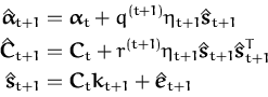
Having the new input, the online updates add one more element
to the
![]() set and the corresponding variables are updated as
set and the corresponding variables are updated as
 |
where we included the updates for the inverse Gram matrix. It was
mentioned in Chapter 2 that the nonzero values at the
t + 1-th elements of the mean and covariance parameters are due to the
t + 1-th unit vector
et + 1. Using this observation, and
comparing the updates with the decomposition of the updated GP
elements from Fig. 3.3, we have
![]() = q(t + 1),
c* = r(t + 1), and
q* =
= q(t + 1),
c* = r(t + 1), and
q* = ![]() . Similarly we identify
the other elements of Fig. 3.3:
. Similarly we identify
the other elements of Fig. 3.3:
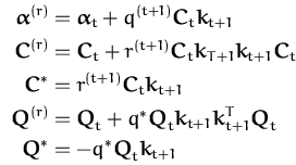 |
and substituting back into the pruning equations (78) and (80) we have
where q* is the last diagonal element of the inverse Gram matrix
Qt + 1,
q* = ![]() = (k* - kt + 1TQtkt + 1)-1. If we use
= (k* - kt + 1TQtkt + 1)-1. If we use
![]() = q*/(q* + r(t + 1)) = (1 +
= q*/(q* + r(t + 1)) = (1 + ![]() r(t + 1))-1 and observe that
Qtkt + 1 =
r(t + 1))-1 and observe that
Qtkt + 1 = ![]() is the projection of the new data
into the subspace spanned by the first t basis vectors, then we
rewrite eq. (87) as
is the projection of the new data
into the subspace spanned by the first t basis vectors, then we
rewrite eq. (87) as
The scalar
![]() can be interpreted as a (re)scaling of the
term
can be interpreted as a (re)scaling of the
term
![]() to compensate for the removal of the last
input. This term again disappears if
to compensate for the removal of the last
input. This term again disappears if
![]() = 0, ie. there is
nothing to compensate for, and the learning rule is the same with the
one described in Section 3.1.
= 0, ie. there is
nothing to compensate for, and the learning rule is the same with the
one described in Section 3.1.
The proposed online GP algorithm is an iterative improvement of the
online learning that assumes an upper limit for the
![]() set. We start
with an empty set and zero values for the parameters
set. We start
with an empty set and zero values for the parameters
![]() and
C. We set the maximal size of the
and
C. We set the maximal size of the
![]() set to d and the prior
kernel to K0. A tolerance parameter
set to d and the prior
kernel to K0. A tolerance parameter
![]() is also used
to prevent the Gram matrix from becoming singular (used in
step 2).
is also used
to prevent the Gram matrix from becoming singular (used in
step 2).
For each element (yt + 1,xt + 1) the algorithm iterates the following steps:
Advance to the next data.
The computational time for a single step is quadratic in d, the
upper limit for the
![]() set. Having an iteration for each data, the
computational time is
set. Having an iteration for each data, the
computational time is
![]() (Nd2). This is a significant
improvement from the
(Nd2). This is a significant
improvement from the
![]() (N3) scaling of the non-sparse GP
algorithms.
(N3) scaling of the non-sparse GP
algorithms.
A computational speedup is to measure the score of the
![]() set
elements and the new data before performing the actual parameter
updates. Since we add a single element, the operations required to
compute the scores are not as costly as the GP updates themselves. If
the smallest score belongs to the new input then we can perform the
sparse update eqs. (88), saving a significant amount
of time.
set
elements and the new data before performing the actual parameter
updates. Since we add a single element, the operations required to
compute the scores are not as costly as the GP updates themselves. If
the smallest score belongs to the new input then we can perform the
sparse update eqs. (88), saving a significant amount
of time.
A further numerical improvement can be made by storing the Cholesky decomposition of the inverse Gram matrix and performing the update and removal operations on the Cholesky decomposition instead of the inverse Gram matrix itself (details can be found in Appendix C.2).
A speedup of the algorithm is possible if we know the
![]() set in
advance: there might be situations where the
set in
advance: there might be situations where the
![]() set is given, e.g
rectangular grid. To implement this we rewrite the prior GP
using the given
set is given, e.g
rectangular grid. To implement this we rewrite the prior GP
using the given
![]() set and a set of GP parameters with all zero
elements:
set and a set of GP parameters with all zero
elements:
![]()
![]() = 0 and
C
= 0 and
C![]() = 0. We then
compute the inverse Gram matrix in advance and if it is not invertible
than we reduce its size by removing the elements having zero distance
= 0. We then
compute the inverse Gram matrix in advance and if it is not invertible
than we reduce its size by removing the elements having zero distance
![]() , an argument discussed at the beginning of this chapter. At
each training step we only need to perform the sparse learning
update rule: to compute the required parameters for the sparse
update of eq. (88) and then to update the parameters.
Testing this simplified algorithm was not done. Since fixing the
, an argument discussed at the beginning of this chapter. At
each training step we only need to perform the sparse learning
update rule: to compute the required parameters for the sparse
update of eq. (88) and then to update the parameters.
Testing this simplified algorithm was not done. Since fixing the
![]() set means fixing the dimension of the data manifold into which we
project our data, an interesting question is the resemblance to Kalman
Filtering (KF) [6]. The KF techniques, originally
from [38,39], are characterised by approximating
the Hessian (i.e. the inverse covariance if using Gaussian pdfs),
together with the values of the parameters. The approximate Hessian
provides a faster convergence of the algorithm possibility to estimate
the posterior uncertainty. The online algorithm for GPs is within the
family of Kalman algorithms, it is an extension to the linear
filtering by exploiting the convenient GP parametrisation from
Chapter 2. For Gaussian regression the two approaches
are the same. However, the extension to the non-standard noise- and
likelihood models is different from the Extended Kalman filtering
(EKF) [24,20]. In EKF the nonlinear model is
linearised using a Taylor expansion around the current parameter
estimates. In applying the online learning we also compute
derivatives, however, the derivative is from the logarithm of the
averaged likelihood [55] instead of the log-likelihood
(EKF case). The averaging makes the general online learning more
robust, we can treat non-differentiable and non-smooth models, an
example is the noiseless classification, presented in
Chapter 5.
set means fixing the dimension of the data manifold into which we
project our data, an interesting question is the resemblance to Kalman
Filtering (KF) [6]. The KF techniques, originally
from [38,39], are characterised by approximating
the Hessian (i.e. the inverse covariance if using Gaussian pdfs),
together with the values of the parameters. The approximate Hessian
provides a faster convergence of the algorithm possibility to estimate
the posterior uncertainty. The online algorithm for GPs is within the
family of Kalman algorithms, it is an extension to the linear
filtering by exploiting the convenient GP parametrisation from
Chapter 2. For Gaussian regression the two approaches
are the same. However, the extension to the non-standard noise- and
likelihood models is different from the Extended Kalman filtering
(EKF) [24,20]. In EKF the nonlinear model is
linearised using a Taylor expansion around the current parameter
estimates. In applying the online learning we also compute
derivatives, however, the derivative is from the logarithm of the
averaged likelihood [55] instead of the log-likelihood
(EKF case). The averaging makes the general online learning more
robust, we can treat non-differentiable and non-smooth models, an
example is the noiseless classification, presented in
Chapter 5.
In this section we compare the sparse approximation from Section 3.3 with other existing methods of dimensionality reduction developed for kernel methods. Most approaches to sparse solutions were developed for the non-probabilistic (and non-Bayesian) case. The aim of these methods is to have an efficient representation of the MAP solution, reducing the number of terms in the representer theorem of [40]. In contrast, the approach in this chapter is a probabilistic treatment of the approximate GP inference, ie. we consider the efficient representability not only of the MAP solution but also of the propagated covariance function.
A first successful algorithm that lead to sparsity within the family
of the kernel methods was the Support Vector Machine (SVM) for the
classification task [93]. This algorithm has gained since
a large popularity and we are not going to discuss it in detail,
instead the reader is referred to available tutorials,
eg. [8] or in [71].3 The SVM algorithm finds the
separating hyperplane in the feature space
![]()
![]() . Due to the
Kimeldorf-Wahba representer theorem we can express the separating
hyperplane using the inputs to the algorithm. Since generally the
separating hyperplane is not unique, in the SVM case further
constraints are imposed: the hyperplane should be such that the
separation is done with the largest possible margin.
. Due to the
Kimeldorf-Wahba representer theorem we can express the separating
hyperplane using the inputs to the algorithm. Since generally the
separating hyperplane is not unique, in the SVM case further
constraints are imposed: the hyperplane should be such that the
separation is done with the largest possible margin.
Furthermore, the cost function for the SVM classification is
non-differentiable, it is the L1 norm of
yi - wTxi for the
noiseless case [93]. This non-differentiable energy
function translates into a inequality constraints over the parameters
![]() and these inequalities lead in turn to sparsity in the
vector
and these inequalities lead in turn to sparsity in the
vector
![]() . The sparsity appears thus only as an indirect
consequence of the formulation of the problem, there is no control
over the ``degree of sparseness'' we want to achieve.
. The sparsity appears thus only as an indirect
consequence of the formulation of the problem, there is no control
over the ``degree of sparseness'' we want to achieve.
An other drawback missing from the SVM formulation is the lack of the probabilities: given a prediction can anything be said about the degree of uncertainty associated with it. There were several attempts to obtain probabilistic SVMs, eg. [62] associated the magnitude of output (in SVM only the sign is taken for prediction) with the certainty level. A probabilistic interpretation of the SVM is presented by [83]: it is shown that, by introducing an extra hyperparameter interpreted as the prior variance of the bias term b in SVM, there exist a Bayesian formulation whose maximum a-posteriori solution leads us back to the ``classical'' support vector machines.
A Bayesian probabilistic treatment in the framework of kernels is also considered by [86]. The starting point of its ``Relevance Vector Machine'' is the extension of the latent function y(x) in terms of the kernel
| y(x) = |
but in this case the coefficients ![]() are random quantities:
each has a normal distribution with a given mean and covariance. The
estimation of the parameters
are random quantities:
each has a normal distribution with a given mean and covariance. The
estimation of the parameters ![]() is transformed thus to the
estimation of the model hyper-parameters consisting of the mean and
variance if the distributions. This is done with an ML-II parameter
estimation and the outcome of this iterative procedure is that many of
the distributions have a diverging variance, effectively eliminating
the corresponding coefficient from the model. The solution is
expressible thus in terms of a small subset of the training data, as
in the SVM case.
is transformed thus to the
estimation of the model hyper-parameters consisting of the mean and
variance if the distributions. This is done with an ML-II parameter
estimation and the outcome of this iterative procedure is that many of
the distributions have a diverging variance, effectively eliminating
the corresponding coefficient from the model. The solution is
expressible thus in terms of a small subset of the training data, as
in the SVM case.
We see thus that for the SVM and RVM case one arrives to sparsity from the definition of the cost function or the model itself. The sparseness in this chapter is of a different nature: we impose constraints on the models themselves and treat arbitrary likelihoods. Three related methods are presented next: the first is the reduction of dimensions using the eigen-decomposition of covariances. The second is the family of the pursuit algorithms that consider the iterative approximation of the model based on a pre-defined dictionary of functions. The last method is related with the original SVM, the Relevance Vector Machines of [86].
Before going into details of specified methods, we mention an other interesting approach to dimensionality reduction: using sampling from mixtures [65]. An infinite mixture of GPs is considered, each GP having an gating network associated. The gating network selects the active GP by which the data will be learnt. It serves as a ``distributor'' of resources when making inference. Although there are possibly an infinite number of GPs that might contribute to the output, in practise the data is allocated to the few different GP experts, easing the problem of inverting a large kernel matrix, technique similar to the block-diagonalisation method of [91].
An established method for reducing the dimension of the data is principal components analysis (PCA) [37]. Since the PCA is also extended to the kernel framework, it is sketched here. It considers the covariance of the data and decomposes it into orthogonal components. If the covariance matrix is C and ui is the set of orthonormal eigenvectors then the covariance matrix is written as
where d is the dimension of the data and furthermore ![]() is
the eigenvalue corresponding to the eigenvector
ui. The
eigenvalues
is
the eigenvalue corresponding to the eigenvector
ui. The
eigenvalues ![]() of the positive (semi)definite covariance
matrix are positive and we can sort them in descending order. The
dimensionality reduction is the projection of the data into the
subspace spanned by the first k eigenvectors. The motivation behind
the projection is that the small eigenvalues and their corresponding
directions are treated as noise. Consequently, projecting
the data to the span of the eigenvectors corresponding to the largest
k eigenvalues will reduce the noise in the inputs.
of the positive (semi)definite covariance
matrix are positive and we can sort them in descending order. The
dimensionality reduction is the projection of the data into the
subspace spanned by the first k eigenvectors. The motivation behind
the projection is that the small eigenvalues and their corresponding
directions are treated as noise. Consequently, projecting
the data to the span of the eigenvectors corresponding to the largest
k eigenvalues will reduce the noise in the inputs.
The kernel extension of the idea of reducing the noise via PCA was studied by [103] (see also [90]). They studied the eigenfunction-eigenvalue equation for the kernel operator:
Since the kernel is positive definite, there are a countable number of eigenfunctions and associated positive eigenvalues. To find the solutions, [103] needed to know the densities of the input in advance. The kernel operator can then be written as a finite or infinite sum of weighted eigenfunctions similarly to eq. (89) (eq. (17) from Section 1.2):
and the solution is specific to the assumed input density, the reason
why we did not use the notation
![]() (x) from
Section 1.2. Arranging the eigenvalues in a descending
order and trimming the sum in eq. (91) leads to an
optimal finite-dimensional feature space. The new kernel can
then be used in any kernel method where the input density has the
given form. The ``projection'' using the eigenfunctions in this case
does not lead directly to a sparse representation in the input space.
The resulting kernel however is finite-dimensional. We have from the
parametrisation lemma that the size of the
(x) from
Section 1.2. Arranging the eigenvalues in a descending
order and trimming the sum in eq. (91) leads to an
optimal finite-dimensional feature space. The new kernel can
then be used in any kernel method where the input density has the
given form. The ``projection'' using the eigenfunctions in this case
does not lead directly to a sparse representation in the input space.
The resulting kernel however is finite-dimensional. We have from the
parametrisation lemma that the size of the
![]() set never has to be
larger than the dimension of the feature space induced by the kernel.
As a consequence, if we are using the modified kernel with the
sparsity criterion developed, the upper limit for the number of
set never has to be
larger than the dimension of the feature space induced by the kernel.
As a consequence, if we are using the modified kernel with the
sparsity criterion developed, the upper limit for the number of
![]() s
set to the truncation of the eq. (91). The input
density is seldom known in advance thus building the optimal
finite-dimensional kernel is generally not possible. A solution was
to replace the input distribution by the empirical distribution of the
data, discussed next.
s
set to the truncation of the eq. (91). The input
density is seldom known in advance thus building the optimal
finite-dimensional kernel is generally not possible. A solution was
to replace the input distribution by the empirical distribution of the
data, discussed next.
The argument of noise reduction was used in kernel PCA
(KPCA) [70] to obtain the nonlinear principal components
of the data. Instead of the analytical form of the input
distribution, the empirical distribution
pemp(x) ![]()
![]()
![]() (xj) was used in the eigenfunction
equation (90) leading to
(xj) was used in the eigenfunction
equation (90) leading to
The eigenfunctions corresponding to nonzero eigenvalues can be
extended using the bi-variate kernel functions at the locations of the
data points
ui(x) = ![]()
![]() K0(xj,x). We can
again use the feature space notation
K0(x,x
K0(xj,x). We can
again use the feature space notation
K0(x,x![]() ) =
) = ![]()
![]() ,
,![]()
![]() . Further we can use
ui(x) =
. Further we can use
ui(x) = ![]()
![]() ,ui
,ui![]() where
ui is an element from the feature
space
where
ui is an element from the feature
space
![]()
![]() , having the form from eq. (93). The
replacement of the input distribution with the empirical one is
equivalent to computing the empirical covariance of the data in the
feature space
Cemp =
, having the form from eq. (93). The
replacement of the input distribution with the empirical one is
equivalent to computing the empirical covariance of the data in the
feature space
Cemp = ![]()
![]()
![]()
![]() .4Equivalently to the problem of eigenfunctions using the empirical
density function, the principal components of the feature space matrix
C corresponding to nonzero eigenvalues are all in the linear span
of
{
.4Equivalently to the problem of eigenfunctions using the empirical
density function, the principal components of the feature space matrix
C corresponding to nonzero eigenvalues are all in the linear span
of
{![]() ,...,
,...,![]() } and can be expressed as
} and can be expressed as
with
![]() i = [
i = [![]() ,...,
,...,![]() ]T the coordinates of
the i-th principal component. The projection of the feature space
images of the data into the subspace spanned by the first k
eigenvectors lead to a ``nonlinear noise reduction''.
]T the coordinates of
the i-th principal component. The projection of the feature space
images of the data into the subspace spanned by the first k
eigenvectors lead to a ``nonlinear noise reduction''.
The dimensionality reduction arising from considering the first k eigenvalues from the KPCA is applied to the kernelised solution provided by the representer theorem. The inputs x are projected to the subspace of the first k principal components
where
![]() (x)Tui is the coefficient corresponding to the
i-th eigenvector. The method, when applied to a subset of size
3000 of the USPS handwritten digit classification problem, showed no
performance loss after removing about 40% of the support
vectors [73]. A drawback of this method is
that although the first k eigenvectors define a subspace of a
smaller dimension than the subspace spanned by all data, to describe
the components the whole dataset is still needed in the
representation of the eigenvectors in the feature space.
(x)Tui is the coefficient corresponding to the
i-th eigenvector. The method, when applied to a subset of size
3000 of the USPS handwritten digit classification problem, showed no
performance loss after removing about 40% of the support
vectors [73]. A drawback of this method is
that although the first k eigenvectors define a subspace of a
smaller dimension than the subspace spanned by all data, to describe
the components the whole dataset is still needed in the
representation of the eigenvectors in the feature space.
A similar approach to KPCA is the Nyström approximation for kernel
matrices applied to kernel methods by [101]. In
the Nyström method a set of reference points is assumed, similarly
to the subspace algorithm from [95]. The true density
function of the inputs in the eigenvalue equation for the kernel,
eq. (90), is approximated with the empirical density
based on the subset
Sm = {x1,...,xm}:
pemp ![]()
![]()
![]() (xi), similarly to the empirical
eigen-system eq. (92), except that Sm is a subset of
the inputs. This leads to the system
(xi), similarly to the empirical
eigen-system eq. (92), except that Sm is a subset of
the inputs. This leads to the system
and the resulting equations are the same as ones from the kernel PCA [70]. The authors then use the first p eigenfunctions obtained by solving eq. (94) to approximate the eigenvalues of the full empirical eigen-system from eq. (92). If we consider all eigenvectors of the reduced eqs. (94), then the approximated kernel matrix is:5
and this identity used in conjunction with the matrix inversion lemma eq. (181) leads to a reduction of the time required to perform the inversion of the kernel Gram matrix KN to a linear scale with the size of the data. An efficient approximation to the full Bayesian posterior for the regression case is straightforward. For classification more approximations are needed, and the Laplace approximation for GPs [99] was implemented leading to iterative solutions to the MAP approximation to the posterior.
Lastly we mention the recent sparse extension of the probabilistic PCA (PPCA) [89] to the kernel framework by [88]. It extends the usual PPCA using the observation that the principal components are expressed using the input data. He considers the parametrisation for the feature-space covariance as
with
![]() the concatenation of the feature vectors for all data and
W a diagonal matrix with the size of the data, this is a
simplification of the representation of the covariance matrix in the
feature space from Section 2.3.1,
eq. (48) using a diagonal matrix instead of the full
parametrisation with respect to the input points. The multiplicative
the concatenation of the feature vectors for all data and
W a diagonal matrix with the size of the data, this is a
simplification of the representation of the covariance matrix in the
feature space from Section 2.3.1,
eq. (48) using a diagonal matrix instead of the full
parametrisation with respect to the input points. The multiplicative
![]() from eq. (96) can be viewed as compensation
for the ignored elements. In the framework of [88] the
value for
from eq. (96) can be viewed as compensation
for the ignored elements. In the framework of [88] the
value for ![]() is fixed and the sparseness is obtained as a
consequence of optimising the KL-divergence between two zero-mean
Gaussians in the feature space. One of them with the empirical
covariance
is fixed and the sparseness is obtained as a
consequence of optimising the KL-divergence between two zero-mean
Gaussians in the feature space. One of them with the empirical
covariance
![]()
![]()
![]() and the other having the
parametrised form of eq. (96). The Gaussian
distributions are considered in the feature space, meaning that the
matrices are of possibly infinite dimensionality. As usual, the
KL-distance can still be expressed with the kernel function and the
parameters
W. The computation of the KL-divergence for the
zero-mean Gaussian distributions is derived in Section 3.2
and the result for zero-means is in eq.(73).
and the other having the
parametrised form of eq. (96). The Gaussian
distributions are considered in the feature space, meaning that the
matrices are of possibly infinite dimensionality. As usual, the
KL-distance can still be expressed with the kernel function and the
parameters
W. The computation of the KL-divergence for the
zero-mean Gaussian distributions is derived in Section 3.2
and the result for zero-means is in eq.(73).
Choosing different values for ![]() will lead to different levels
of sparsity. On the top of sparsity, the diagonal matrix is a
significant reduction in the number of parameters. The drawback of
this method is that it requires an iterative solution for finding the
diagonal matrix
W. The iterations require the kernel matrix with
respect to all data.
will lead to different levels
of sparsity. On the top of sparsity, the diagonal matrix is a
significant reduction in the number of parameters. The drawback of
this method is that it requires an iterative solution for finding the
diagonal matrix
W. The iterations require the kernel matrix with
respect to all data.
The efficient representation is an important issue in the family of kernel methods, thus the diagonalisation of the covariance parameter might lead to significant increase in the speed of the GP algorithms. We discussed the diagonalisation of matrix C in conjunction with the online learning rule in Appendix E. It leads to a system that, unlike the simple update rules from eq. (57) using a full matrix to parametrise the covariance in the feature space, cannot be solved exactly, instead we are required to develop an iterative procedure to find the new diagonal matrix Ct + 1 given the GP parameters from time t and the new data. In addition to the possible iterations each time a new data is included, the system requires the manipulation of a full matrix to obtain Ct + 1. It turns out that there are no exact updates and we have to use a second, embedded loop for getting the solution which renders the approach extremely difficult computationally. The conclusion is that the diagonalisation is not feasible if used within the framework of the online learning. Additionally, it would be interesting to test the loss caused by diagonalising the sparse GP solution find by the sparse online algorithm presented in this chapter.
Based on the kernel-PCA decomposition of the kernel matrix, first we mention the ``reduced set'' method was developed by [73]. The full SVM solution is sparsified by removing a single element or a group of elements. The updates and the loss are computed when removing a single element or a group (the loss is similar to the simplified KL-divergence of eq. (85), more discussions there).
A generic ``subspace'' algorithm for the family of kernel methods was proposed by [95, Chapter 7]. The projection into the subset is implemented with the set of basis elements fixed in advance, the projection is made exploiting the linearity of the feature space (as presented in Section 3.1) and it is applied to the MAP solution of the problem.
The reduced approximation for the kernel matrix as shown in eq. (95) has also been used for regression [79,80]. They also address the question of choosing the m-dimensional subset of the data in detail. The selection criterion is based on the examination of each input contributing to the kernel matrix and an approximation of the error made by not including the specific column. In a sequential algorithm the most important columns (and rows) are included into the basis set. Our sparse GP approximation uses the same philosophy of examining the ``score'' of the individual inputs iterative addition (section 3.4). Instead of concentrating to the MAP solutions, as it is done in the methods sketched, a full probabilistic treatment is considered in this thesis.
The sparse greedy Gaussian process regression, as shown in [79], is similar to a family of established pursuit methods: projection pursuit [35] and basis pursuit [12,11]. The pursuit algorithms consider a set of functions, this set is usually called a dictionary. The assumption is that using all elements from the dictionary is not feasible: there might be infinitely many elements in the dictionary. An other situation is when the dictionary is over-complete, i.e. a function has more then one representation using this dictionary. The task is then to choose a subset of functions that give good solutions to the problem. The solution is given in the form of a linear combination of elements from the dictionary, and the optimal parameters given the selected functions are found similarly to the generalised linear models, presented in Chapter 1.
Considering problem of choosing the optimal subset from a dictionary, in the kernel methods we use the data both as the training examples to the algorithm (data in a conventional sense) but at the same time, due to the representer theorem, the dictionary of the available functions is also specified by the same data set. This is the case both for the non-probabilistic solution, given by the representer theorem and for the representation of the GPs, result given in Chapter 2. The efficient construction of a subset in the kernel methods is thus equivalent with the sparse representation, the topic of this chapter. The pursuit literature deals with the selection of basis from a non-probabilistic viewpoint, here we consider a fully probabilistic treatment of selecting the dictionary.
In [94] the pursuit algorithms is combined with the kernel methods in their work: ``Kernel matching pursuit''. They address the selection of the inputs - this time viewed as elements from a dictionary - and the optimal updates of the coefficients of the kernelised solutions to the problem.
In the basic matching pursuit the individual elements from the dictionary are added one by one. Once a dictionary element is taken into the set representing the solutions, in the basic version of the pursuit algorithms, its weighting coefficient is not changed. This is suboptimal solution if we want to keep the size of the elements from the dictionary as small as possible. A proposed solution is the ``orthogonal matching pursuit'', or ``back-fitting'' algorithm where the next dictionary elements is chosen by optimising in the whole subspace of the functions chosen so far. This implies recomputing the weights for each function already chosen in the previous steps. This can be derived using linear algebra [94].
Looking at the online update eqs. (57) we see that the updates implemented correspond to the back-fitting approach. This optimal update in our case uses the second order information stored in the covariance matrix, or equivalently, the parameters C of the covariance. The scores (Section 3.4) when removing an element also chooses a subspace - thus is a restrictive solution - into which to project the solutions. The choice of the subspace is based on varying all parameters to find the projection. The parameter updates are optimal in the KL-sense and update all coefficients, similarly to the case of back-fitting for the kernel matching pursuit or the orthogonal matching pursuit [60].
The difference between the matching pursuit algorithms and the
sparsity in GPs is the use of KL-based measures for the kernel family,
implying a full probabilistic treatment. At the same time, using the
online learning in conjunction with the sparsity presented here leads
to a greedier algorithm than the pursuit algorithms, this is because
in the iterative process of obtaining the solution only those inputs
are considered that are in the sparse
![]() set, i.e. the dictionary.
This leads to a removal of some inputs that might be relevant if all data would be considered when removing a
set, i.e. the dictionary.
This leads to a removal of some inputs that might be relevant if all data would be considered when removing a
![]() .
.
This chapter considered the optimal removal of a data point from the representation of a Gaussian process, where the optimality is measured using the KL-divergence.
The KL-optimal projection that leads to sparseness, as it is defined in Section 3.3 does not depend on the algorithm used for obtaining the non-sparse solution. This is important, saying that the idea of ``sparsifying solutions'' is not restricted to the online learning alone. However, we found that the combination of sparsity with the online learning results in a robust algorithm with a non-increasing size of the parameter set.
An important feature of the algorithm is that the basis vectors for
representing the GP are selected during runtime from the data. This
was possible due to the computationally cheap evaluation of the error
made if current input was not included into, or a previous input was
removed from the
![]() set. It is important that the error, i.e. the
score of an element from the
set. It is important that the error, i.e. the
score of an element from the
![]() set from eq. (83)
and (85), did not require the effective computation
of the pruned GP, rather we were able to express it based solely on
the already available elements. This is similar to the leave-one-out
error [96] within the probabilistic framework of
Gaussian processes.
set from eq. (83)
and (85), did not require the effective computation
of the pruned GP, rather we were able to express it based solely on
the already available elements. This is similar to the leave-one-out
error [96] within the probabilistic framework of
Gaussian processes.
For real applications the sparsity combined with the online method has
an additional benefit: the iterative computation of the inverse Gram
prevents the set of basis vectors from being redundant: when the new
input is in the linear span of the
![]() set, this vector is replaced by
its representation using the previous vectors.
set, this vector is replaced by
its representation using the previous vectors.
The benefit of the sparse GP algorithm is its inherent Bayesian probabilistic treatment of the inference. This allows an efficient approximation to the posterior kernel of the process which in turn leads to estimating the predictive variance. Thus we can quantify the quality of the prediction.
The memory requirement of the reduced GP is quadratic in the size of
the
![]() set. The possibility for further reduction might be
important. A further reduction of the parameters where the full
matrix
C was replaced with a diagonal one has been also examined
(see Appendix E), similarly to the kernel extension of
the probabilistic PCA algorithm (PPCA) [88]. We found
however that, as in the case of PPCA, there was no exact solution to
the KL-optimal projection, instead of it, we are required to perform
iterative EM-like optimisation. This severely affects the speed of the
algorithm and was not pursued further.
set. The possibility for further reduction might be
important. A further reduction of the parameters where the full
matrix
C was replaced with a diagonal one has been also examined
(see Appendix E), similarly to the kernel extension of
the probabilistic PCA algorithm (PPCA) [88]. We found
however that, as in the case of PPCA, there was no exact solution to
the KL-optimal projection, instead of it, we are required to perform
iterative EM-like optimisation. This severely affects the speed of the
algorithm and was not pursued further.
The algorithm also has a few shortcomings. First, it is a greedy algorithm: at a certain moment the pruning of the GPs only considers the inputs that were selected at previous times. The GP will thus possibly be biased toward the last elements: they may be over-represented. Another problem is that the solution depends on the ordering of the data that is arbitrary, a possible solution to this will be considered in the next chapter.
The sparse online algorithm from Section 3.6 cannot do batch-like processing of the data by processing it multiple times. For large datasets this is not a problem, but for smaller data set sizes we might want to have a second sweep through the data. A solution to this is proposed in the next chapter by combining the sparse algorithm with the ``expectation-propagation'' algorithm, an extension of the online iterations from Chapter 2 to allow multiple iterations [46].
We also did not consider the problem of outliers. These types of data
seriously damage the performance of the algorithms. The Bayesian
framework is less sensitive to the outliers in general. However, the
removal of a
![]() implies that the resulting algorithm is just an
approximation to the true Bayesian solution. More important, in the
sparse GP case the scores for the inputs are largest for outliers. To
ensure a good performance for the sparse algorithm, we will probably
need to pre-process the data by first removing the outliers.
implies that the resulting algorithm is just an
approximation to the true Bayesian solution. More important, in the
sparse GP case the scores for the inputs are largest for outliers. To
ensure a good performance for the sparse algorithm, we will probably
need to pre-process the data by first removing the outliers.
It would be interesting to test the performance of the online learning algorithm if we allow an ordering of the data according to the possible gain of information from learning the specific data instance. For this we can use the KL-distance from eq. (75):
| 2KL( |
and we see that for the computation of the KL-distance we do not
need to do the update of the GP parameters. We can compute this
quantity in
![]() (Np2) time for all untrained data and let the
``most informative'' data be processed first.
(Np2) time for all untrained data and let the
``most informative'' data be processed first.
We could also extend the sparse GP learning algorithm to query learning. In query learning only a fraction of the total data is labelled and the labelling of the examples is costly. This might be the case in the chemical industry or pharmaceutics where there are high costs for each experiment to label the data.
We want to improve thus our algorithm by learning the data which is the most informative given our assumptions about the model and the already labelled examples. This is an intensely researched area, called active- or query learning. Using tools from statistical physics and making specific assumptions, results for both classification [75] and regression [82], and extending it to non-parametric family is an interesting research topic.
For classification, the symmetry of the cost or likelihood function is
exploited. It is thus possible to compute the KL-divergence between
the current GP and the one that would be obtained if a data
(xl, yl) were processed with only the knowledge that yl is
binary. For this we see that the KL-distance from
eq. (75) for the classification case does not
depend on the output label. Recent study for the Support Vector
classification was made by [9] and they showed
increased performance when applied to real dare. Testing this idea
for the GPs and comparing with other methods of query learning is an
interesting future project. It would be interesting to propose methods
that do not rely (solely) on the KL-distance, but rather on increases
in the generalisation ability of the system (as it was proposed
in [82]).
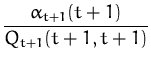
![$\displaystyle ({\boldsymbol { \alpha } }_2 - {\boldsymbol { \alpha } }_1)^T
\le...
...l { K } }_B \right]
({\boldsymbol { \alpha } }_2 - {\boldsymbol { \alpha } }_1)$](img323.png)
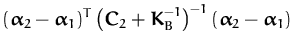
![\begin{displaymath}\begin{split}& \ensuremath{\mathrm{tr}}\left[({\boldsymbol { ...
...{ C } }_2+{\boldsymbol { K } }_B^{-1})^{-1} \right] \end{split}\end{displaymath}](img326.png) .
. trAn
trAn![$\displaystyle \ln\left\vert {\boldsymbol { I } }_{\ensuremath{\pmb{\cal{F}}}}+ ...
...\Sigma } }}_2^{-1} - {\boldsymbol { I } }_{\ensuremath{\pmb{\cal{F}}}}\right]^n$](img329.png)
![$\displaystyle - \sum_{n=1}^\infty \frac{(-1)^n}{n}
\ensuremath{\mathrm{tr}}\lef...
...l { C } }_2)({\boldsymbol { C } }_2+{\boldsymbol { K } }_B^{-1})^{-1} \right]^n$](img330.png)

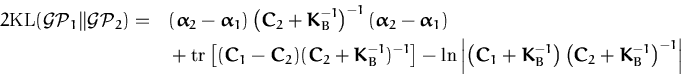 .
.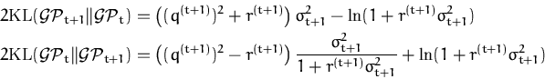
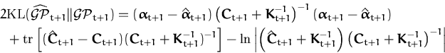

 -
- 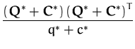
![\includegraphics[]{decomp.eps}](img371.png)
 -
-  -
- 
![\includegraphics[]{non-agree-fr1-all.eps}](img395.png)
![\includegraphics[]{non-agree-fr1-50and0.9.eps}](img396.png)