In obtaining sparsity in eqs. (78)
and (80), we need the inverse Gram matrix of the
![]() set.
In the following the elements of the
set.
In the following the elements of the
![]() set are indexed from 1 to
t. Using the matrix inversion formula, eq. (182), the
addition of a new element is done sequentially. This is well known,
commonly used in the Kalman filter algorithm. We consider the new
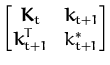
element at the end (last row and column) of matrix
Kt + 1. The
matrix
Kt + 1 is decomposed:
set are indexed from 1 to
t. Using the matrix inversion formula, eq. (182), the
addition of a new element is done sequentially. This is well known,
commonly used in the Kalman filter algorithm. We consider the new
element at the end (last row and column) of matrix
Kt + 1. The
matrix
Kt + 1 is decomposed:
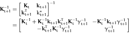
Assuming Kt-1 known and applying the matrix inversion lemma for Kt + 1:
where
![]() = k*t + 1 - kt + 1TKt-1kt + 1 is
the squared distance of the last feature vector from the linear span
of all previous ones (see Section 3.1). Using notations
Kt-1kt + 1 =
= k*t + 1 - kt + 1TKt-1kt + 1 is
the squared distance of the last feature vector from the linear span
of all previous ones (see Section 3.1). Using notations
Kt-1kt + 1 = ![]() from eq. (62),
Kt-1 = Qt, and
Kt + 1-1 = Qt + 1 we have the recursion:
from eq. (62),
Kt-1 = Qt, and
Kt + 1-1 = Qt + 1 we have the recursion:
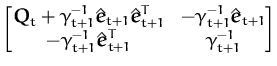
and in a more compact matrix notation:
where
et + 1 is the t + 1-th unit vector. With this recursion
equation all matrix inversion is eliminated (this result is general
for block matrices, such implementation, together with an
interpretation of the parameters has been also made
in [10]). The introduction of the rule
![]() > 0 guarantees non-singularity of the Gram matrix (see
Fig. 3.1).
> 0 guarantees non-singularity of the Gram matrix (see
Fig. 3.1).
The block-diagonal decomposition of the Gram matrix from eq. (188) allows us to have a recursive expression for the determinant. Using eq. (184), we have
where
![]() is the squared distance of the new input from the
subspace spanned by all previous inputs.
is the squared distance of the new input from the
subspace spanned by all previous inputs.
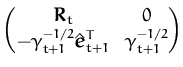
For numerical stability we can use the Cholesky-factorisation of the inverse Gram matrix Q. Using the lower-triangular matrix R with the corresponding indices, and the identity Q = RTR, we have the update for the Cholesky-decomposition
that is a computationally very inexpensive operation, without
additional operations provided that the quantities
![]() and
et + 1 are already computed.
and
et + 1 are already computed.
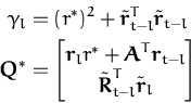
In Chapter 3 the diagonal elements of the inverse
Gram matrix are used in establishing the score for an element of the
![]() set, and the columns of the same Gram matrix are used in updating
the GP elements. Fixing the index of the column to l, we have the
l-th diagonal element and the columns expressed as
set, and the columns of the same Gram matrix are used in updating
the GP elements. Fixing the index of the column to l, we have the
l-th diagonal element and the columns expressed as
where we used the decomposition of Rt + 1 along the l-th column
Rdatat + 1 = 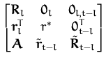 |
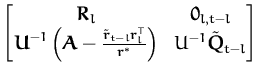
and the update of the Cholesky decomposition, when removing the l-th column is written as
with U being the Cholesky decomposition of
IN - l +  . This is always positive definite and there
is a fast computation for U (in matlab one can compute it with
U=cholupdate(I,qN/q) with corresponding quantities).
. This is always positive definite and there
is a fast computation for U (in matlab one can compute it with
U=cholupdate(I,qN/q) with corresponding quantities).