We want to find the constrained GP with parameters
(![]() ,
,![]() ) with the last elements all having
zero values (see Section 3.3) that minimises the
KL-divergence
) with the last elements all having
zero values (see Section 3.3) that minimises the
KL-divergence
and we suppose the GP parameters
(![]() t + 1,Ct + 1) and the
t + 1,Ct + 1) and the
![]() set are given (we know
Kt + 1 and
Kt). In the following
we use
Kt + 1-1 = Qt + 1 and the decomposition of the
GP parameters as presented in Chapter 3, with
Fig 3.3 repeated in Fig D.1.
set are given (we know
Kt + 1 and
Kt). In the following
we use
Kt + 1-1 = Qt + 1 and the decomposition of the
GP parameters as presented in Chapter 3, with
Fig 3.3 repeated in Fig D.1.
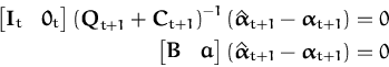
The differentiation with respect to parameters
![]() ,...,
,...,![]() leads to the system of
equations that is easily written in matrix form as
leads to the system of
equations that is easily written in matrix form as
where It is the identity matrix and 0t is the column vector of length t with zero elements. In the second line the matrix multiplication has been performed and we used the decomposition
Finally, using the decomposition of the vector
![]() t + 1 from
Fig. 3.3, we have
t + 1 from
Fig. 3.3, we have
and
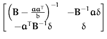
![]() is obtained from the matrix inversion lemma
for block matrices from eq. (182). Using the matrix
inversion lemma for
(Qt + 1 + Ct + 1)-1 from
eq. (198) we have:
is obtained from the matrix inversion lemma
for block matrices from eq. (182). Using the matrix
inversion lemma for
(Qt + 1 + Ct + 1)-1 from
eq. (198) we have:
and using the correspondence
![]() = q* + c* and
Q* + C* = - B-1a
= q* + c* and
Q* + C* = - B-1a![]() read from eq. (199), we have
read from eq. (199), we have
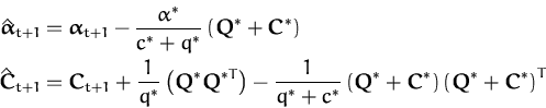
and replacing it into the expression for the reduced mean parameters, we have
![]()
Before differentiating the KL-divergence with respect to
![]() , we simplify the terms that include
, we simplify the terms that include
![]() in eq. (196). Firstly we write the
constraints for the last row and column of
in eq. (196). Firstly we write the
constraints for the last row and column of
![]() using the
extension matrix
[It 0t] as
using the
extension matrix
[It 0t] as
where
![]() is a matrix with t rows and columns,
and in the following we will use
is a matrix with t rows and columns,
and in the following we will use
![]() instead of
instead of
![]() . Permuting the elements in the trace term of
eq. (196) leads to
. Permuting the elements in the trace term of
eq. (196) leads to
where the additive term
- Ct + 1(Ct + 1 + Qt + 1)-1 is
ignored since it will not contribute to the result of the
differentiation. Ignoring also the term not depending on
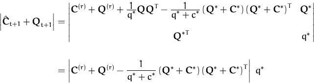
![]() in the determinant, and using the replacement of
in the determinant, and using the replacement of
![]() from eq. (202) we simplify the
log-determinant
from eq. (202) we simplify the
log-determinant
where we used the decomposition into block-diagonal matrices (first line) and the expression for the determinants of block-diagonal matrices from eq (184).
The differentiation of the KL-distance with respect to
![]() is the addition of differentiating
eqs. (203) and (204):
is the addition of differentiating
eqs. (203) and (204):
We apply the matrix inversion lemma to the RHS similarly to the case of eq (204) and retaining only the upper-left part leads to
and the reduced covariance parameter is
![]()
ARRAY(0x896d3ec)ARRAY(0x896d3ec)
We are assessing the error made when pruning the GP by evaluating the
KL-divergence from eq. (196) between the process with
(![]() t + 1,Ct + 1) and the pruned one with
(
t + 1,Ct + 1) and the pruned one with
(![]() ,
,![]() ) from the previous section. We
start by writing the pruning equations in function of
t + 1-dimensional vectors: in the following we will use
Q*
) from the previous section. We
start by writing the pruning equations in function of
t + 1-dimensional vectors: in the following we will use
Q* ![]() [Q*Tq*]T and
C*
[Q*Tq*]T and
C* ![]() [C*Tc*]T and the pruning
equations are
[C*Tc*]T and the pruning
equations are
and it is easy to check that the updates will result in the last row and column being all zeros. In computing the KL-divergence we will use the identities from the matrix algebra:
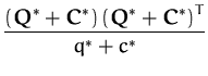
Based on the first identity, the term containing the mean is
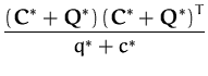
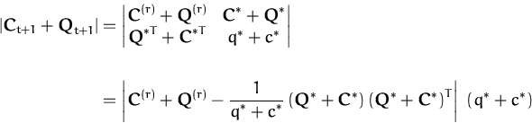
The logarithm of the determinants is transformed, using the determinants of the block-diagonal matrices, in eq. (184):
and using a similar decomposition for the denominator we have
and the logarithm of the ratio has the simple expression as
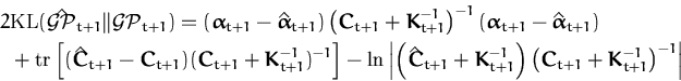
Finally, using the invariance of the trace of a product with respect
to circular permutation of its elements, the trace term is:
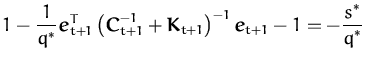
where s* is the last diagonal element of the matrix (Ct + 1-1 + Kt + 1)-1. Summing up eqs (209), (212), and (213), we have the minimum KL-distance
Matrix inversion is a sensitive issue and we are trying to avoid it.
In computing the score for a given
![]() in the previous section,
eq. (214), we need the diagonal element of the
matrix
S = (C-1 + K)-1. In this section we sketch an
iterative update rule for the matrix
S, and an update when the
KL-optimal removal of the last
in the previous section,
eq. (214), we need the diagonal element of the
matrix
S = (C-1 + K)-1. In this section we sketch an
iterative update rule for the matrix
S, and an update when the
KL-optimal removal of the last
![]() element is performed.
element is performed.
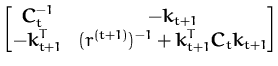
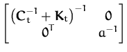
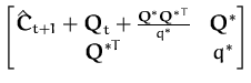
First we establish the update rules for the inverse of matrix Ct + 1. By using the matrix inversion lemma and the update from eq. (57), the matrix C-1 is
then we combine the above relation with the block-diagonal decomposition of the kernel matrix, and observing that the t×1 column vector is zero, we have
 where a = (r(t + 1))-1 + kt + 1TCtkt + 1 + k* where a = (r(t + 1))-1 + kt + 1TCtkt + 1 + k* |
and this shows that the update for the matrix St + 1 is particularly simple: we only need to add a value on the last diagonal element.
When removing a
![]() however, the resulting matrix will not be diagonal
any more. To have an update quadratic in the size of
S, we use the
matrix inversion lemma
however, the resulting matrix will not be diagonal
any more. To have an update quadratic in the size of
S, we use the
matrix inversion lemma
| St + 1 = Qt + 1 - Qt + 1 |
and after the pruning we are looking for the t×t matrix
![]() =
= ![]()
![]() + Kt
+ Kt![]() . We
can obtain this by using eq. (206): the pruned
. We
can obtain this by using eq. (206): the pruned
![]()
![]() + Qt
+ Qt![]() is the matrix obtained
by cutting the last row and column from
is the matrix obtained
by cutting the last row and column from
![]() Ct + 1 + Qt + 1
Ct + 1 + Qt + 1![]() . The computation of the
updated matrix
. The computation of the
updated matrix
![]() has thus three steps:
has thus three steps:
![\includegraphics[]{decomp.eps}](img371.png)

 with
with 

![$\displaystyle \ensuremath{\mathrm{tr}}\left[\hat{{\boldsymbol { C } }}_{t+1}
\b...
...{bmatrix}{\boldsymbol { I } }_t & {\boldsymbol { 0 } }_t\end{bmatrix}^T
\right]$](img846.png)
 -
-  -
- 


![$\displaystyle \frac{1}{q^*}{\boldsymbol { Q } }^{*T}\left[{\boldsymbol { K } }_...
...}_{t+1}\right)^{-1}
{\boldsymbol { K } }_{t+1} \right]{\boldsymbol { Q } }^* -1$](img883.png)