Modelling with Gaussian processes (GPs) has received increased attention in the machine learning community. A formal definition of the GPs is that of a collection of random variables fx having a (usually) continuous index where any finite collection of the random variables has a joint Gaussian distribution [15]. The realisation of a GP is a random function f (x) = fx specified by the mean and covariance function of the GP.
Inference with GPs is non-parametric since the ``parameters'' to be
learnt are the mean and covariance functions describing
fx.
The function
fx is used as a latent variable in a likelihood
P(y|x, fx) which denotes the probability of an observable output
variable y given the input
x. For the inference using GPs, we
only need to specify the prior mean and the prior covariance functions
of
fx, the latter is called the kernel
K0(x,x![]() ) = Cov(fx, fx
) = Cov(fx, fx![]() ) [95]. The prior mean
function is usually the zero function, thus the choice of the kernel fully
specifies the GP. Having the training data
{(xn, yn)}n = 1N, the
posterior process for
fx is obtained from the prior and the
likelihood using the Bayesian approach [3,98], as
outlined in Section 1.2.
) [95]. The prior mean
function is usually the zero function, thus the choice of the kernel fully
specifies the GP. Having the training data
{(xn, yn)}n = 1N, the
posterior process for
fx is obtained from the prior and the
likelihood using the Bayesian approach [3,98], as
outlined in Section 1.2.
There are two major obstacles in implementing this theoretically simple Bayesian inference: non-Gaussianity of the posteriors and the size of the kernel matrix K0(xi,xj). In this chapter we consider the problem of representing the non-Gaussian posterior, and an intuitive KL-based approximation to reduce the size of the kernel matrix is proposed in Chapter 3.
Obtaining analytical results in GP inference is precluded by the non-tractable integrals in the posterior averages, the normalisation from eq. (2). Various methods have been introduced to approximate these averages. A variety of such methods may be understood as approximations of the non-Gaussian posterior process by a Gaussian one [36,74], for instance in [99] the posterior mean is replaced by the posterior maximum (MAP) and information about the fluctuations are derived by a quadratic expansion around this maximum.
The modelling approach proposed here is also an approximation to the posterior GP and uses the likelihood to obtain predictions. For this we need to represent the posterior GP using a finite number of parameters. This parametrisation is possible for the moments of the posterior process. Based on minimising a KL-distance, the parametrisation proposed for the posterior GP uses the form provided by the posterior mean and kernel functions. This form of the parametrisation does not depend on the likelihood model we are using, thus the particular likelihood will be left unspecified. Since we are propagating Gaussians, the framework presented suits unimodal likelihood functions. Using multi-modal likelihoods, as in Section 5.4 is not theoretically difficult but the quality of approximation is poorer.
This chapter starts by introducing GPs using generalised linear models, in Section 2.1 and the Bayesian learning applied to GPs in Section 1.2. We then deduce the parametrisation for the posterior moments, one of the main contributions of this thesis in Section 2.3. Based on the parametrisation we derive the online learning rules for approximating the posterior process in Section 2.4 and the chapter ends with a short discussion.
For an illustration of Bayesian learning from Section 1.1 we consider the problem of quadratic regression with additive Gaussian noise. This problem is analytically tractable and will be used in subsequent chapters to illustrate different aspect of the deduced algorithms. The likelihood for a single example is
with ![]() the variance of the noise and function
f (x,
the variance of the noise and function
f (x,![]() )
specifying the class of regressors to be used. The prior over the
parameters
)
specifying the class of regressors to be used. The prior over the
parameters
![]() is Gaussian with zero mean and spherical
covariance
is Gaussian with zero mean and spherical
covariance
![]() . Applying Bayes rule from
eq. (3) leads to the posterior probability for the
parameters
. Applying Bayes rule from
eq. (3) leads to the posterior probability for the
parameters
![]() :
:
In generalised linear models [44] the function
f (x) is a linear combination of k functions
{![]() (x)}i = 1k, called the function dictionary:
(x)}i = 1k, called the function dictionary:
with model coefficients
![]() . We introduce the more compact
vectorial notation
. We introduce the more compact
vectorial notation
![]() x = [
x = [![]() (x),...,
(x),...,![]() (x)]T.
Since GPs can be obtained by a further generalisation step of the
generalised linear models, we introduce the basic notation in this
section; this notation is used in later chapters.
(x)]T.
Since GPs can be obtained by a further generalisation step of the
generalised linear models, we introduce the basic notation in this
section; this notation is used in later chapters.
The Gaussian data likelihood is the product of the individual
likelihoods from eq. (12) and leads to a Gaussian
posterior obtained by using eq. (13). To express the
posterior, we group the values of the dictionary function
![]() x
for all data in the matrix
x
for all data in the matrix
![]() = [
= [![]() x1,...,
x1,...,![]() xN], introduce the bivariate
kernel function
K(x,x
xN], introduce the bivariate
kernel function
K(x,x![]() ) =
) = ![]()
![]()
![]() (x)
(x)![]() (x
(x![]() ) =
) = ![]()
![]() xT
xT![]() x
x![]() , and build the N×N matrix
KN =
, and build the N×N matrix
KN = ![]() K(xr,xs)
K(xr,xs)![]() . With these notations
the mean and covariance of the posterior distribution, after an
algebraic rearrangement of eq. (12), is:
. With these notations
the mean and covariance of the posterior distribution, after an
algebraic rearrangement of eq. (12), is:
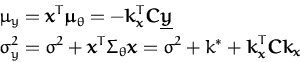
where we used the notation
![]() = [y1,...,yN]T and
C = -
= [y1,...,yN]T and
C = - ![]()
![]() IN + KN
IN + KN![]() . The latter notation,
used for the the posterior covariance, is rather complicated, but this
is the form it appears later in this chapter
(section 2.4, page
. The latter notation,
used for the the posterior covariance, is rather complicated, but this
is the form it appears later in this chapter
(section 2.4, page ![]() ) for the general
non-parametric case.
) for the general
non-parametric case.
Similarly to the posterior, the predictive distribution of the output
f (x) = y given the input
x has also a Gaussian distribution,
denoted
![]() with parameters
with parameters
where ![]() is the noise variance and we used
kx = [K(x,x1),..., K(x,xN)]T and
k* = K(x,x) for the
kernel products. Note that
is the noise variance and we used
kx = [K(x,x1),..., K(x,xN)]T and
k* = K(x,x) for the
kernel products. Note that
![]() was included into the kernel
K, thus it is not explicit in eq. (16).
was included into the kernel
K, thus it is not explicit in eq. (16).
General Gaussian processes are obtained from extending the Bayesian
learning for the generalised linear models to a large set of basis
functions. We can use arbitrarily large, even infinite dictionaries
{![]() (x)}i = 1
(x)}i = 1![]() in building the approximation from
eq. (14). For the predictive distribution we only need to
specify the kernel function
K(x,x
in building the approximation from
eq. (14). For the predictive distribution we only need to
specify the kernel function
K(x,x![]() ), i.e. the covariance of the
random variables
f (x) and
f (x
), i.e. the covariance of the
random variables
f (x) and
f (x![]() ):
):
where we considered different variances
![]() for the random
variables
for the random
variables ![]() .
.
We can choose the dictionary and the variances of the normal random
variables freely, however this choice would only change the kernel
K(x,x![]() ). In GPs we only consider the kernels and ignore the
possible dictionaries that might have generated it. Using the kernels
provides larger flexibility: as long as the sum
K(x,x
). In GPs we only consider the kernels and ignore the
possible dictionaries that might have generated it. Using the kernels
provides larger flexibility: as long as the sum
K(x,x![]() ) from
eq. (17) converges, the dictionary is not
important, it can be any countable set.
) from
eq. (17) converges, the dictionary is not
important, it can be any countable set.
The condition for
K(x,x![]() ) to be used as a kernel function is to
generate a valid covariance matrix for any input set
) to be used as a kernel function is to
generate a valid covariance matrix for any input set ![]() : the
matrix
KN is positive definite for arbitrary set of inputs,
i.e. the kernel function is positive definite. It has been
shown that any positive definite kernel function can be written, using
Mercer's theorem [93,71], in the form of
eq. (17), thus they indeed can be viewed as being
generated from a family of generalised linear models. The difference
is that for kernels the size of the function dictionary does not need
to be finite. Using infinite dictionaries, e.g. the dense family of
RBF kernels, within the maximum likelihood estimation leads to
over-fitting, this is not the case for the Bayesian parameter
estimation method. In this case setting priors over the weights acts
like regularisation [85,63], preventing
over-fitting.
: the
matrix
KN is positive definite for arbitrary set of inputs,
i.e. the kernel function is positive definite. It has been
shown that any positive definite kernel function can be written, using
Mercer's theorem [93,71], in the form of
eq. (17), thus they indeed can be viewed as being
generated from a family of generalised linear models. The difference
is that for kernels the size of the function dictionary does not need
to be finite. Using infinite dictionaries, e.g. the dense family of
RBF kernels, within the maximum likelihood estimation leads to
over-fitting, this is not the case for the Bayesian parameter
estimation method. In this case setting priors over the weights acts
like regularisation [85,63], preventing
over-fitting.
In the following we illustrate the decomposition of kernels into dictionary functions using two popular kernels: the polynomial and the radial basis kernel.
Let us first consider one-dimensional inputs and the dictionary for
the generalised linear model be
![]() 1,
1,![]() x,x2
x,x2![]() with random variables
{
with random variables
{![]() }i = 13 all having zero means and
unit variances. The random functions drawn from this model have the
form
f (x) =
}i = 13 all having zero means and
unit variances. The random functions drawn from this model have the
form
f (x) = ![]() +
+ ![]()
![]() x +
x + ![]() x2 and we have
the kernel as
x2 and we have
the kernel as
| K(x,x |
To find the functions and priors corresponding to the RBF kernels we will proceed in the opposite direction: we are considering the Taylor expansion of the exponential in the RBF kernel:
where we have
![]() (x) = exp(- x2/(2
(x) = exp(- x2/(2![]() ))xn and
))xn and
![]() = 1/(n!2
= 1/(n!2![]() )n and we can indeed see that the RBF
kernel has a set of corresponding basis of functions with infinite
cardinality. It is also obvious that by rescaling each component with
)n and we can indeed see that the RBF
kernel has a set of corresponding basis of functions with infinite
cardinality. It is also obvious that by rescaling each component with
![]() , we have a spherical Gaussian prior for the parameter
vector
, we have a spherical Gaussian prior for the parameter
vector
![]() , a vector that will have infinitely many elements.
, a vector that will have infinitely many elements.
It is important to mention that the decomposition of the kernels in
pairs of feature spaces and associated scalar products is not unique.
The quadratic polynomial kernel for example can be written using a set
of dictionary with four elements:
![]() 1,x,x,x2
1,x,x,x2![]() and requiring four random variables.
and requiring four random variables.
Different embedding spaces for the RBF kernels can also be considered. For example a decomposition to an orthonormal set of functions with respect to an input measure has been employed in [103]. The decomposition was used to prune the components of the infinite sum in eq. (17) to obtain a finite-dimensional linear model. The pruning considered only the most important dictionary functions and the result was a low-dimensional representation that kept as much information about the model as it was possible.
In kernel methods the dictionary of the kernel defines the feature space
![]()
![]() . Assuming we have k functions in the
dictionary, the feature space is
. Assuming we have k functions in the
dictionary, the feature space is
![]() k and the projection
function is defined by
k and the projection
function is defined by
![]() (x) = [
(x) = [![]()
![]() (x),...]T.
Using the projection function
(x),...]T.
Using the projection function ![]() and the feature space
and the feature space
![]()
![]() ,
,
![]() (x) =
(x) = ![]() is the image of the input
x in the feature
space and then the kernel function is
is the image of the input
x in the feature
space and then the kernel function is
where we concatenate the outputs of the different ![]() -s into a
vector. The kernel functions can then be viewed as scalar products of
the projections from the input space to the feature space
-s into a
vector. The kernel functions can then be viewed as scalar products of
the projections from the input space to the feature space
![]() and the
easiest way to gain insight into the kernel algorithms is by looking
at the (usually) simpler linear algorithm in the feature space.
and the
easiest way to gain insight into the kernel algorithms is by looking
at the (usually) simpler linear algorithm in the feature space.
The generalised linear model for the regression is tractable, however, the problem now is computational: usually the number of inputs is much higher than k, the number of parameters of the model. This implies that a direct inversion of matrix C for computing the predictive distribution is inefficient. For the class of generalised linear models with finite dictionary there are efficient methods to find the predictive distribution, we can exploit that KN is not a full-rank matrix. For the non-parametric GPs, discussed next, the rank of KN generally equals the size of the data. This implies that matrix C cannot be inverted efficiently, and the problem of cubic computational time cannot be avoided.
In the following we will use GPs as priors with the prior kernel
K0(x,x![]() ): an arbitrary sample
f from the GP at spatial
locations
): an arbitrary sample
f from the GP at spatial
locations
![]() = [x1,...,xN]T has a Gaussian
distribution with covariance
K
= [x1,...,xN]T has a Gaussian
distribution with covariance
K![]() :
:
Using
f![]() = {f (x1),..., f (xN)} for the
random variables at the data positions, we compute the posterior
distribution as
= {f (x1),..., f (xN)} for the
random variables at the data positions, we compute the posterior
distribution as
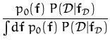
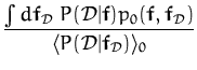
where
p0(f,f![]() ) is the joint Gaussian distribution of
the random variables at the training and sample locations,
) is the joint Gaussian distribution of
the random variables at the training and sample locations,
![]() P(
P(![]() |f
|f![]() )
)![]() is the average of the likelihood with respect to
the prior GP marginal,
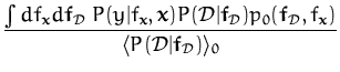
p0(f). Computing the predictive
distributions is the combination of the posterior with the likelihood
of the data at
x
is the average of the likelihood with respect to
the prior GP marginal,
p0(f). Computing the predictive
distributions is the combination of the posterior with the likelihood
of the data at
x
The analytic treatment is possible only for regression with Gaussian noise, which is presented next. The different approximation techniques to the posterior are given in Section 2.2.2
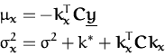
For regression we can immediately read from eq. (16) the predictive distribution corresponding to input x. It is a Gaussian with mean and covariance given by
where
![]() is the vector of observed (noisy) outputs,
k(x) = [K0(x,x1),..., K0(x,xN)]T,
k* = K0(x,x),
C = - (
is the vector of observed (noisy) outputs,
k(x) = [K0(x,x1),..., K0(x,xN)]T,
k* = K0(x,x),
C = - (![]() I + KN)-1 with
KN the kernel matrix of the data, and
I + KN)-1 with
KN the kernel matrix of the data, and ![]() . This is the same as
eq. (16) for the generalised linear models from
Section 1.1.
. This is the same as
eq. (16) for the generalised linear models from
Section 1.1.
|
Figure 2.1 shows the result of the GP learning with a
polynomial and an RBF kernel. The function we approximate is the noisy
![]() function
function
![]() (continuous line) where
(continuous line) where ![]() is a zero mean Gaussian noise of variance
is a zero mean Gaussian noise of variance
![]() = 0.2, noise
variance assumed to be known. For this illustration we had equidistant
inputs (dots) from the interval [- 4, 2.5] and we plotted the mean and
deviation of the predictive marginal distributions from the interval
[- 4, 4]. We see that due to the localised nature of the RBF kernels,
the predictive uncertainty of the model is increasing in the regions
where there are no input data (the right part of
Fig 2.1.a). In contrast, when polynomial kernels are
used, due to their non-localised kernel, the variance does not
increase significantly outside the input region, providing a worse
model. The differences can also be understood by comparing the
supports for the two classes of kernels. Polynomial kernel has an
infinite support, i.e. each data has effect over the whole input
region. In contrast, the support of the RBF kernel is practically
vanishing after a certain distance from the origin, depending on the
value of the kernel parameters. This means that the RBF kernel is
better suited to modelling the
= 0.2, noise
variance assumed to be known. For this illustration we had equidistant
inputs (dots) from the interval [- 4, 2.5] and we plotted the mean and
deviation of the predictive marginal distributions from the interval
[- 4, 4]. We see that due to the localised nature of the RBF kernels,
the predictive uncertainty of the model is increasing in the regions
where there are no input data (the right part of
Fig 2.1.a). In contrast, when polynomial kernels are
used, due to their non-localised kernel, the variance does not
increase significantly outside the input region, providing a worse
model. The differences can also be understood by comparing the
supports for the two classes of kernels. Polynomial kernel has an
infinite support, i.e. each data has effect over the whole input
region. In contrast, the support of the RBF kernel is practically
vanishing after a certain distance from the origin, depending on the
value of the kernel parameters. This means that the RBF kernel is
better suited to modelling the
![]() function when the width of the
RBF function being set appropriately. The 6-th order polynomial
gives a crude estimation in this case.
function when the width of the
RBF function being set appropriately. The 6-th order polynomial
gives a crude estimation in this case.
The GP regression is impossible for large datasets since the matrix C from eq. (23) has the number of columns and rows equal to the size of the dataset and we need an inversion to obtain it. Easing this computational load was considered by [26]: the predictive mean from eq (23) was iteratively approximated using conjugate gradient minimisation of the quadratic form
with respect to
u. Since
Q(u) is quadratic, the conjugate
gradient algorithm will converge to the true minima
- Cy after
N steps, and results at any previous stage constitute approximations
to
- Cy (again, due to the notation,
C-1 is the known
entity). A lower and an upper bound for the error based on
eq. (24) has also been proposed, this gave a
stopping criterion to the algorithm. Optimising simultaneously a pair
of quadratic forms with a first one in eq. (24)
and a second, slightly different function:
Q*(u) = yTKNu + ![]() uTC-1KNu was studied
by [78]. The simultaneous optimisation of the quadratic
forms also provides a stopping criterion by combining the values of
the two quadratic forms.
uTC-1KNu was studied
by [78]. The simultaneous optimisation of the quadratic
forms also provides a stopping criterion by combining the values of
the two quadratic forms.
The Bayesian committee machine [91] provides a different
approach to avoid the inversion of large matrices. The assumptions
made in this case is that the data is clustered into subsets
![]() = {
= {![]() 1,...,
1,...,![]() p}. In probabilistic terms this
means that for any two subsets the conditional probabilities of the
outputs factorise, i.e.
p(fq|
p}. In probabilistic terms this
means that for any two subsets the conditional probabilities of the
outputs factorise, i.e.
p(fq|![]() i,
i,![]() i + 1)
i + 1) ![]() p(fq)p(
p(fq)p(![]() i|fq)p(
i|fq)p(![]() i + 1|fq), or practically
that
C has a block-diagonal structure. This leads to p
subproblems of smaller size and the combination of the subproblems
into predicting a unique value is done using Bayes' rule. This
approximation however might not perform well, since in large system
there could be the case that, although the off-diagonal elements are
not individually significant, the overall or cumulated effect cannot
be neglected without a significant loss.
i + 1|fq), or practically
that
C has a block-diagonal structure. This leads to p
subproblems of smaller size and the combination of the subproblems
into predicting a unique value is done using Bayes' rule. This
approximation however might not perform well, since in large system
there could be the case that, although the off-diagonal elements are
not individually significant, the overall or cumulated effect cannot
be neglected without a significant loss.
In addition to the constraint imposed by large matrices for the regression case, a full Bayesian treatment of GPs using other likelihoods requires approximations to the models, presented next.
An approximation to the intractable posterior distribution is via sampling. Markov-chain Monte-Carlo methods have been used to sample from GP posteriors for regression and classification [49]. Sampling was employed in the application of GPs for classification in ``Bayes Point Machines'' by [32]: the resulting solution is the centre of mass of the version space, i.e. the space of all acceptable solutions for the classification. Sampling methods from a posterior obtained from a model inversion problem using Gaussian processes as priors has been considered [47] with the aim of finding the wind-fields underlying the scatterometer measurement (see Section 5.4 for details). The different sampling techniques are applicable to a large class of methods, however they are extremely time-demanding: the dimension of the space from which we are sampling is high, and in addition, it is hard to establish the convergence of algorithms. In what follows we will focus on analytic approximations.
For classification, the logistic function is one possibility to be used in the likelihood
and this makes the GP posterior from eq. (21) analytically intractable. Several approximations have been thoroughly studied. A Laplace approximation around the MAP solution was suggested in [99] where the Hessian and the approximation of the data likelihood led to the possibility of modifying the kernel function for the GP. A Laplace approximation and multiple iterations when predicting for an unknown value are also needed.
A different approach is to use variational approximations to the
logistic function to perform the required
averages [36,27]. The logistic
function is approximated with exponentials having free variational
parameters ![]() for each input as
for each input as
with
![]() (
(![]() ) a known function. Since the GP marginals are
different for different inputs, the variational parameter
) a known function. Since the GP marginals are
different for different inputs, the variational parameter ![]() needs to be computed for each input. The approximation involves the
optimisation with respect to the set of variational parameters
needs to be computed for each input. The approximation involves the
optimisation with respect to the set of variational parameters
![]() , a computationally demanding task, requiring iterative
optimisation. For prediction, an additional optimisation with respect
to a variational parameter
, a computationally demanding task, requiring iterative
optimisation. For prediction, an additional optimisation with respect
to a variational parameter
![]() is required.
is required.
Based on the variational methods, approximations can also be found via
the minimisation of the KL divergence [14]. Having two
distributions
p(![]() ) and
q(
) and
q(![]() ) of the random variable
) of the random variable
![]() , the KL divergence is defined as
, the KL divergence is defined as
The KL divergence is used to approximate the posterior distribution arising from Bayes rule with a distribution belonging to a tractable class.
The KL measure is not symmetric in its arguments,
thus we have two possibilities to use it. Let ![]() denote the
approximating distribution and ppost be the intractable
posterior. Minimising
denote the
approximating distribution and ppost be the intractable
posterior. Minimising
![]() with respect to
with respect to
![]() requires expectations to be carried only over the tractable
distribution
requires expectations to be carried only over the tractable
distribution ![]() ; this variational method in the context of
Bayesian neural networks was called ensemble
learning [33,1]. The KL distance is written
as
; this variational method in the context of
Bayesian neural networks was called ensemble
learning [33,1]. The KL distance is written
as
where the first term is the negative entropy term of the approximating distribution. The approximations usually belong to the exponential family, thus an exact integration is often possible. For mixture models the integration over the log-posterior is also intractable, a common substitution is made via the log-sum inequality, leading to an upper bound for the log-posterior [76].
A variational approximation to the full posterior process was proposed
by [74] where the intractable posterior from
eq (21) is approximated using a Gaussian with mean
![]() and a covariance matrix
and a covariance matrix
![]() = D +
= D + ![]() ciciT with
D a diagonal matrix and
ci additional parameters of the
covariance [4]. This joint Gaussian distribution is for
the parameters
ciciT with
D a diagonal matrix and
ci additional parameters of the
covariance [4]. This joint Gaussian distribution is for
the parameters
![]() of the MAP solutions the to
posterior [40,93]
of the MAP solutions the to
posterior [40,93]
This equation is the posterior mean if GP priors are used
(see [57] and Section 2.3 for details),
and efficient approximations within the mean-field framework were
given [17]. The approximating distribution there was a
factorising one
![]() q(fi) and the parameters for the
individuals were obtained by computing the KL divergence between the
posterior and the factorised distributions, leading to approximations
for the coefficients
q(fi) and the parameters for the
individuals were obtained by computing the KL divergence between the
posterior and the factorised distributions, leading to approximations
for the coefficients
![]() from eq. (28).
Additionally to the solution for the prediction problem, the
variational framework provided bounds and approximations to the model
likelihood, opening the possibility to optimise the hyper-parameters
of the model.
from eq. (28).
Additionally to the solution for the prediction problem, the
variational framework provided bounds and approximations to the model
likelihood, opening the possibility to optimise the hyper-parameters
of the model.
We can interchange the terms in the non-symmetric KL measure and try to optimise the ``reversed'' (compared to ensemble learning eq. (27)) KL divergence
The important difference compared to the measure in eq. (27) is that the approximating distribution appears only once and, more important, the averaging is done with respect to the exact posterior distribution. Analytic expression for the posterior is not available, generally this choice leads to equally difficult approximation problems.
If one interprets the KL divergence as the expectation of the relative
log loss of two distributions, this choice of divergence weights the
losses with the correct distribution rather than with the approximated
one. A second observation is that the variation of
eq. (29) with respect to ![]() involves only the
second term, the entropy of the posterior distribution (first term)
being independent of the parameters used for approximation, whilst in
the other case the entropy of the approximation needed to be
considered.
involves only the
second term, the entropy of the posterior distribution (first term)
being independent of the parameters used for approximation, whilst in
the other case the entropy of the approximation needed to be
considered.
We will use this latter distance measure to approximate the
intractable posterior. Since we are dealing with Gaussian processes,
hence normal distributions, the ``tractable''
![]() (
(![]() ) will
be Gaussian. Denoting the mean and covariance of
) will
be Gaussian. Denoting the mean and covariance of ![]() with
with
![]() and
and
![]() respectively, the KL divergence is
respectively, the KL divergence is
where B is a constant that does not depend on the unknown parameters
of ![]() . Differentiating eq. (30) with respect to
the parameters
. Differentiating eq. (30) with respect to
the parameters
![]() and
and
![]() gives us the mean and
covariance of the intractable posterior [55], then
setting the differentials to zero leads to
gives us the mean and
covariance of the intractable posterior [55], then
setting the differentials to zero leads to
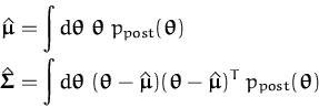
Thus, if the distance measure is chosen to be eq. (29), then the resulting approximation is the matching of the moments of the posterior process. However, the posterior distribution eq. (21) used for expressing posterior expectations in eq. (31) requires the evaluation of typically high dimensional integrals. This is also true for prediction, when we are interested in expectations of functions of the process at inputs which are not contained in the training set. Even if we had good methods for approximate integration, this would make predictions a rather tedious task. For a single data or if we can reduce our problem to one-dimensional integrals, there are several applicable approximations, both analytic and look-up table based. This has lead to the idea of online learning that iteratively approximates the posterior distribution by using a single data at every processing step [54]. This iterative approximation to the posterior, also called projection to a tractable family, will be discussed in Section 2.4 later in this chapter.
In the following the parametric model is replaced by the
non-parametric GPs and the parameter vector
![]() by a random
function
f (x). The non-parametric case can be treated similarly
to the parametric one, we will refer to the non-parametric case as
consisting of ``any finite collection'' of parameters. To apply the
online learning for the non-parametric GPs, we need to find a
convenient representation for the posterior moments. We will
establish a ``parametrisation'' to the posterior moments that uses a
number of parameters growing with the size of the data - this being
the definition of non-parametric methods - presented next.
by a random
function
f (x). The non-parametric case can be treated similarly
to the parametric one, we will refer to the non-parametric case as
consisting of ``any finite collection'' of parameters. To apply the
online learning for the non-parametric GPs, we need to find a
convenient representation for the posterior moments. We will
establish a ``parametrisation'' to the posterior moments that uses a
number of parameters growing with the size of the data - this being
the definition of non-parametric methods - presented next.
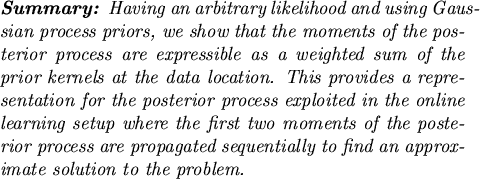
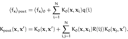
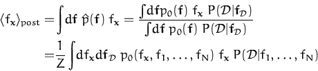
The predictive distribution of eq. (22), as it is presented, might require the computation of a new integral each time a prediction on a novel input is required. The following lemma shows that simple but important predictive quantities like the posterior mean and the posterior covariance of the process at arbitrary inputs can be expressed as a combination of a finite set of parameters which depend on the process at the training data only. Knowing these parameters eliminates the high-dimensional integrations when we are doing predictions.
Based on the rules for partial integration we provide a representation
for the moments of the posterior process obtained using GP priors and
a given data set ![]() . The property used in this chapter is
that of Gaussian averages: for a differentiable scalar function
g(x) with
x
. The property used in this chapter is
that of Gaussian averages: for a differentiable scalar function
g(x) with
x ![]()
![]() d, based on the partial integration
rule [30], we have the following relation
(Th. 1 on page
d, based on the partial integration
rule [30], we have the following relation
(Th. 1 on page ![]() ):
):
where the function
g(x) and its derivatives grow slower than an
exponential to guarantee the existence of the integrals involved. We
use the vector integral to have a more compact and more intuitive
formulation and
![]() g(x) is the vector of derivatives. The
vector
g(x) is the vector of derivatives. The
vector
![]() is the mean and matrix
is the mean and matrix
![]() is the covariance of
the normal distribution p0. To keep the text more clear, the proof
is postponed to Appendix B.
is the covariance of
the normal distribution p0. To keep the text more clear, the proof
is postponed to Appendix B.
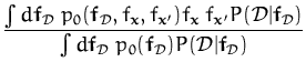
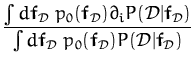
The context in which eq. (32) is useful is when p0(x) is a Gaussian and g(x) is a likelihood. We want to compute the moments of the posterior [57,17]. For arbitrary likelihoods we can show that
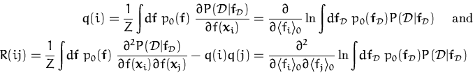
The parameters q(i) and R(ij) are given by
where
f![]() = [f (x1),..., f (xN)]T and
Z =
= [f (x1),..., f (xN)]T and
Z = ![]() df p0(f)P(
df p0(f)P(![]() |f
|f![]() ) is a normalising constant and the
partial differentiations are with respect to the prior mean at
xi.
) is a normalising constant and the
partial differentiations are with respect to the prior mean at
xi.
 |
where
f is a set of realisations for the random process indexed
by arbitrary points from
![]() m, the inputs for the GPs.
m, the inputs for the GPs.
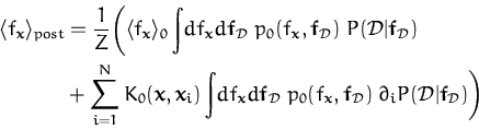
We compute first the mean function of the posterior process:
where the denominator was denoted by Z, we used the vectorial
notation
f![]() = [f1,..., fN]T, and we also used the
short notation
f (x) = fx and
f (xi) = fi. Observe that,
irrespectively of the number of the random variables of the process
considered, the dimension of the integral we need to consider is
only N + 1, all other random variables will be marginalised. We
thus have an N + 1-dimensional integral in the numerator and Z is
an N-dimensional integral. If we group the variables related to
the data as
f
= [f1,..., fN]T, and we also used the
short notation
f (x) = fx and
f (xi) = fi. Observe that,
irrespectively of the number of the random variables of the process
considered, the dimension of the integral we need to consider is
only N + 1, all other random variables will be marginalised. We
thus have an N + 1-dimensional integral in the numerator and Z is
an N-dimensional integral. If we group the variables related to
the data as
f![]() = [f1,..., fN]T, and apply the
property of Gaussian averages from eq. (32) (also
eq. (185) from Appendix B) replacing
x by
fx and
g(x) by
P(
= [f1,..., fN]T, and apply the
property of Gaussian averages from eq. (32) (also
eq. (185) from Appendix B) replacing
x by
fx and
g(x) by
P(![]() |f
|f![]() ), we have
), we have
where K0 is the kernel function generating the covariance matrix
(
![]() in Theorem. 1). The variable
fx in the
integrals disappears since it is only contained in p0.
Substituting back the normalising factor Z leads to the expression
of the posterior mean as
in Theorem. 1). The variable
fx in the
integrals disappears since it is only contained in p0.
Substituting back the normalising factor Z leads to the expression
of the posterior mean as
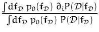
where qi is read off from eq. (36)
It is clear that the coefficients qi depend only on the data, and are independent of the point x at which the posterior mean is evaluated.
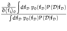
We will simplify the expression for qi by performing a change of
variables in the numerator:
f'i = fi - ![]() fi
fi![]() where
where
![]() fi
fi![]() is the prior mean at
xi and keeping all other
variables unchanged
f'j = fj, j
is the prior mean at
xi and keeping all other
variables unchanged
f'j = fj, j ![]() i, leading to the numerator
i, leading to the numerator
and
![]() is the differentiation with respect to the new
variables f'i. Since they are related additively, we can replace
the partial differentiation with respect to f'i with the partial
differentiation with respect to the mean
is the differentiation with respect to the new
variables f'i. Since they are related additively, we can replace
the partial differentiation with respect to f'i with the partial
differentiation with respect to the mean
![]() fi
fi![]() . Since the
differentiation and integral operators apply for a distinct set of
variables, we can swap their order to have
. Since the
differentiation and integral operators apply for a distinct set of
variables, we can swap their order to have
 |
where
![]() /
/![]()
![]() fi
fi![]() is the differentiation with
respect to the mean of the prior GP at
xi. We then perform the
inverse change of variables inside the integral and substitute back
into the expression for qi
is the differentiation with
respect to the mean of the prior GP at
xi. We then perform the
inverse change of variables inside the integral and substitute back
into the expression for qi
For the posterior covariance we follow a similar way. Using posterior averages, the kernel is expressed as:
and we can use the results from eq. (37) for the
last term in the above equation. For the first average we apply the
property of the Gaussian averages with
g(f, fx![]() ) = fx
) = fx![]() P(
P(![]() |f
|f![]() ) and using the posterior process from
eq. (21), we have
) and using the posterior process from
eq. (21), we have
The summation in the second term is over the data set ![]() and the second input index
x
and the second input index
x![]() . The notation
. The notation
![]() stands for the differentials with respect to
fxi and
fx
stands for the differentials with respect to
fxi and
fx![]() , the random variable
fx
, the random variable
fx![]() can be viewed as an
additional data point at this stage. We split the sum in two parts,
making explicit the term including
x
can be viewed as an
additional data point at this stage. We split the sum in two parts,
making explicit the term including
x![]() , the derivative of
g(f, fx
, the derivative of
g(f, fx![]() ) with respect to
fx
) with respect to
fx![]() being
P(
being
P(![]() |f
|f![]() ) and
cancelling the denominator,
this leads to
) and
cancelling the denominator,
this leads to
and we apply again Theorem 1
(eq. (32)) to each term of the sum where function
g(f![]() ) =
) = ![]() P(
P(![]() |f
|f![]() ); the last term is transformed
as
); the last term is transformed
as
where the second line is just a rearrangement of the first one. All we have to do now is to substitute back the resulting formulae in the equation for the posterior moment (40). Using qi from eq. (37) leads to the expression for the posterior kernel to
where Dij is
and we can use the replacement in the differentiation where the
random variable
fxi is replaced with the prior mean
![]() fxi
fxi![]() , using a similar procedure to that used for the
first moment from eq. (38) to eq. (39).
Identifying
Rij = Dij - qiqj leads to the required
parametrisation in equation (34) from
Lemma 2.3.1. Simplification of
Rij = Dij - qiqj is
made by changing the arguments of the partial derivative and using
the logarithm of the expectation (repeating
steps (38)-(39) made to obtain qi),
leading to
, using a similar procedure to that used for the
first moment from eq. (38) to eq. (39).
Identifying
Rij = Dij - qiqj leads to the required
parametrisation in equation (34) from
Lemma 2.3.1. Simplification of
Rij = Dij - qiqj is
made by changing the arguments of the partial derivative and using
the logarithm of the expectation (repeating
steps (38)-(39) made to obtain qi),
leading to
and this concludes the proof.
![]()
The parametric form of the posterior mean, eq. (33), resembles the representation eq. (6) for other kernel approaches like the Support Vector Machines, that are obtained by minimising certain cost functions such as the negative log-posterior or the regularised linear models. These results are attractive, and they provide a representation for the solution of an optimisation problem that can be regarded as a maximum-likelihood solution (MAP) to the full Bayesian representation.
While the latter representations are derived from the representer theorem of [40] (generalised in [72]) our result from eq. (33) does, to our best knowledge not follow from this, but is derived from simple properties of Gaussian distributions. To have a probabilistic treatment for the problem, we need a representation for the full posterior distribution, and this has not been provided in the representer theorem.
The representation lemma plays an important role in providing basis for the online learning, presented in Section 2.4. It also serves as a basis for the reduced representation (sparsity in Chapter 3) and, in addition to the non-probabilistic Support Vector Machines, in the applications we are able to compute the Bayesian error bars for the prediction.
We also stress that the parameters q(i) and R(ij) have to be computed only once, in the training phase: they are fixed when we make predictions. The bad news is that the analytic computation of the parameters however is in most cases impossible. Apart from the lack of analytic tractability, the equations for the posterior moments require the computation of an integral having the dimension of the data. A solution to overcome the large computational difficulty is to build a sequential method for approximating the parameters, called online learning [54,55].
Before presenting the online learning for the GPs, let us describe a different perspective to the parametrisation lemma.
The parametrisation lemma provides us the first two moments of the
posterior process. Apart from the Gaussian regression, where the
results are exact, we can consider the moments of the posterior
process as approximations. This approximation is written in a
data-dependent coordinate system. We are using the feature space
![]()
![]() and the projection
and the projection
![]() of the input
x into
of the input
x into
![]()
![]() . With the
scalar product from eq. (19) replacing the kernel
function K0, we have the mean and covariance functions for the
posterior process as
. With the
scalar product from eq. (19) replacing the kernel
function K0, we have the mean and covariance functions for the
posterior process as
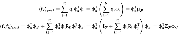
This shows that the mean function is expressed in the feature space as
a scalar product between two quantities: the feature space image of
x and a ``mean vector''
![]() , also a feature-space entity. A
similar identification for the posterior covariance leads to a
covariance matrix in the feature space that fully characterises the
covariance function of the posterior process.
, also a feature-space entity. A
similar identification for the posterior covariance leads to a
covariance matrix in the feature space that fully characterises the
covariance function of the posterior process.
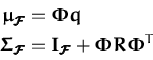
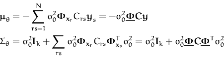
The conclusion is the following: there is a correspondence of the
approximating posterior GP with a Gaussian distribution in the
feature space
![]()
![]() where the mean and the covariance are expressed as
where the mean and the covariance are expressed as
with the concatenation of the feature vectors for all data.
This result provides us with the interpretation of the Bayesian GP inference as a family of Bayesian algorithms performed in a feature space and the result projected back into the input space by expressing it in terms of scalar products. Notice two important additions to the kernel method framework given by the parametrisation lemma:
The main difference between the Bayesian GP learning and the non-Bayesian kernel method framework is that, in contrast to the approaches based on the representer theorem for SVMs which result in a single function, the parametrisation lemma gives a full probabilistic approximation: we are ``projecting'' back the posterior covariance in the input space.
Also an important observation is that the parametrisation is
data-dependent: both the mean and the covariance are expressed in a
coordinate system where the axes are the input vectors ![]() and
q and
R are coordinates for the mean and covariance
respectively. Using once more the equivalence to the generalised
linear models from Section 2.2, the GP approximation to
the posterior GP is a Gaussian approximation to
and
q and
R are coordinates for the mean and covariance
respectively. Using once more the equivalence to the generalised
linear models from Section 2.2, the GP approximation to
the posterior GP is a Gaussian approximation to
![]() .
.
A probabilistic treatment for the regression case has been recently proposed [88] where the probabilistic PCA method [89,67] is extended to the feature space. The PPCA in the kernel space uses a simpler approximation to the covariance which has the form
where the ![]() takes arbitrary values and
W is a diagonal matrix of the size of the data. This is a special case of
the parametrisation lemma of the posterior GP
eq. (48). This simplification leads to a sparseness.
This is the result of an EM-like algorithm that minimises the
KL distance between the empirical covariance in the feature space
takes arbitrary values and
W is a diagonal matrix of the size of the data. This is a special case of
the parametrisation lemma of the posterior GP
eq. (48). This simplification leads to a sparseness.
This is the result of an EM-like algorithm that minimises the
KL distance between the empirical covariance in the feature space
![]()
![]()
![]() and the parametrised covariance of
eq. (49), a more detailed discussion is delayed to
Section 3.7. The minimisation of the KL distance
can also seen as a special case of the online learning, that will be
presented in the next section.
and the parametrised covariance of
eq. (49), a more detailed discussion is delayed to
Section 3.7. The minimisation of the KL distance
can also seen as a special case of the online learning, that will be
presented in the next section.
In the following the joint normal distribution in the feature space with the data-dependent parametrisation from eq. (48) will be used to deduce the sparsity in the GPs.
The representation lemma shows that the posterior moments are expressed as linear and bilinear combinations of the kernel functions at the data points. On the other hand, the high-dimensional integrals needed for the coefficients q = [q1,..., qN]T and R = {Rij} of the posterior moments are rarely computable analytically, the parametrisation lemma thus is not applicable in practise and more approximations are needed.
The method used here is the online approximation to the posterior distribution using a sequential algorithm [55]. For this we assume that the data is conditionally independent, thus factorising
and at each step of the algorithm we combine the likelihood of a
single new data point and the (GP) prior from the result of the
previous approximation step [17,58]. If
![]() denotes the Gaussian approximation after processing t
examples, by using Bayes rule we have the new posterior process
ppost given by
denotes the Gaussian approximation after processing t
examples, by using Bayes rule we have the new posterior process
ppost given by
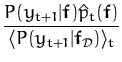
Since ppost is no longer Gaussian, we approximate it with the
closest GP,
![]() (see Fig. 2.2). Unlike the
variational method, in this case the ``reversed'' KL divergence
(see Fig. 2.2). Unlike the
variational method, in this case the ``reversed'' KL divergence
![]() from eq. (29) is minimised.
This is possible, because in our on-line method, the posterior
(51) only contains the likelihood for a single data
and the corresponding non-Gaussian integral is one-dimensional. For
many relevant cases these integrals can be performed analytically or
we can use existing numerical approximations.
from eq. (29) is minimised.
This is possible, because in our on-line method, the posterior
(51) only contains the likelihood for a single data
and the corresponding non-Gaussian integral is one-dimensional. For
many relevant cases these integrals can be performed analytically or
we can use existing numerical approximations.
![\includegraphics[]{online.eps}](img218.png)
|
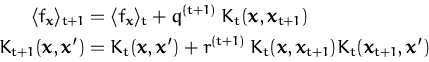
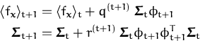
In order to compute the on-line approximations of the mean and covariance kernel Kt we apply Lemma 2.3.1 sequentially with a single likelihood term P(yt| ft,xt) at each step. Proceeding recursively, we arrive at
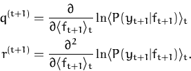
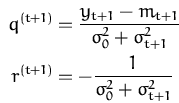
where the scalars q(t + 1) and r(t + 1) follow directly from applying Lemma 2.3.1 with a single data likelihood P(yt + 1|xt + 1, fxt + 1) and the process from time t:
where ``time'' is referring to the order in which the individual
likelihood terms are included in the approximation. The averages in
(53) are with respect to the Gaussian process at
time t and the derivatives taken with respect to
![]() ft + 1
ft + 1![]() =
= ![]() f (xt + 1)
f (xt + 1)![]() . Note again, that these averages only require
a one dimensional integration over the process at the input xt + 1.
. Note again, that these averages only require
a one dimensional integration over the process at the input xt + 1.
The online learning eqs. (52) in the feature space have the simple from [55]:
and this form of the online updates will be used in Chapter 4 to extend the online learning to an iterative fixed-point algorithm.
Unfolding the recursion steps in the update rules (52)
we arrive at the parametrisation for the approximate posterior GP at
time t as a function of the initial kernel and the likelihoods:
with coefficients
![]() (i) and Ct(ij) defining the approximation to the posterior process, more precisely to its
coefficients
q and
R from eq. (33) and
equivalently in eq. (48) using the feature space. The
coefficients given by the parametrisation lemma and those provided by
the online iteration eqs. (55) and (56) are
equal in the Gaussian regression case only. The approximations are
given recursively as
(i) and Ct(ij) defining the approximation to the posterior process, more precisely to its
coefficients
q and
R from eq. (33) and
equivalently in eq. (48) using the feature space. The
coefficients given by the parametrisation lemma and those provided by
the online iteration eqs. (55) and (56) are
equal in the Gaussian regression case only. The approximations are
given recursively as
where kt + 1 = kxt + 1 = [K0(xt + 1,x1),..., K0(xt + 1,xt)]T and et + 1 = [0, 0,..., 1]T is the t + 1-th unit vector.
We prove eqs. (55) and (56) by induction: we
will show that for every time-step we can express the mean and kernel
functions with coefficients
![]() and
C,which are functions
only of the data points
xi and kernel function K0 and do not
depend on the values
x and
x
and
C,which are functions
only of the data points
xi and kernel function K0 and do not
depend on the values
x and
x![]() at which the mean and kernel
functions are computed.
at which the mean and kernel
functions are computed.
Proceeding by induction and using the induction hypothesis
![]() 0 = C0 = 0 for time t = 1, we have
0 = C0 = 0 for time t = 1, we have
![]() (1) = q(1)
and
C1(1, 1) = r(1). The mean function at time t = 1 is
(1) = q(1)
and
C1(1, 1) = r(1). The mean function at time t = 1 is
![]() fx
fx![]() =
= ![]() (1)K0(x1,x) (from lemma 2.3.1
for a single data, eq. (52)). Similarly the modified
kernel is
K1(x,x
(1)K0(x1,x) (from lemma 2.3.1
for a single data, eq. (52)). Similarly the modified
kernel is
K1(x,x![]() ) = K0(x,x
) = K0(x,x![]() ) + K(x,x1)C1(1, 1)K0(x1,x
) + K(x,x1)C1(1, 1)K0(x1,x![]() ) with
) with
![]() and
C independent of
x and
x
and
C independent of
x and
x![]() , thus proving the induction hypothesis.
, thus proving the induction hypothesis.
We assume that at time t we have the parameters
![]() t
and
Ct independent of the points
x and
x
t
and
Ct independent of the points
x and
x![]() and the mean
and kernel functions expressed according to eq. (55)
and (56) respectively. The update for the mean can then
be written as
and the mean
and kernel functions expressed according to eq. (55)
and (56) respectively. The update for the mean can then
be written as
| = | |||
| + q(t + 1)K0(x,xt + 1) | |||
| = | |||
| = | (58) |
where
![]() t + 1 does not involve the input
x and the update
is as in eq. (57). Writing down the update
equation for the kernels
t + 1 does not involve the input
x and the update
is as in eq. (57). Writing down the update
equation for the kernels
| Kt + 1(x,x |
|||
| r(t + 1) |
|||
| = K0(x,x |
|||
| = K0(x,x |
(59) |
where in the elements of
Ct + 1 are independent of
x and
x![]() and we can read off the updates for the elements of the matrix
Ct + 1 easily. In summary, we have the recursions for the GP
parameters in vectorial notation from eqs. (58)
and (59). Replacing
and we can read off the updates for the elements of the matrix
Ct + 1 easily. In summary, we have the recursions for the GP
parameters in vectorial notation from eqs. (58)
and (59). Replacing
![]() with the t + 1-th
unit vector
et + 1 we obtain the recursion equations
eq (57).
with the t + 1-th
unit vector
et + 1 we obtain the recursion equations
eq (57).
![]()
To illustrate the online learning we consider the case of
regression with Gaussian noise (variance
![]() ), presented
in Section 1.1. At time t + 1 we need the
one-dimensional marginal of the GP parametrised with
(
), presented
in Section 1.1. At time t + 1 we need the
one-dimensional marginal of the GP parametrised with
(![]() t,Ct), the marginal being taken at the new data point
xt + 1. This marginal is a normal distribution with mean
mt + 1 = kt + 1T
t,Ct), the marginal being taken at the new data point
xt + 1. This marginal is a normal distribution with mean
mt + 1 = kt + 1T![]() t and covariance
t and covariance
![]() = k* + kt + 1TCtkt + 1. The next step is to
compute the logarithm of the average likelihood
= k* + kt + 1TCtkt + 1. The next step is to
compute the logarithm of the average likelihood
ln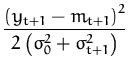 |
and the first and second derivatives with respect to the mean mt + 1 give the scalars q(t + 1) and r(t + 1):
 |
Comparing the update equations with the exact results for regression,
we have
![]() t = - Ct
t = - Ct![]() and
Ct = - (
and
Ct = - (![]() I + Kt)-1, this is identical to the case of
generalised linear models (section 2.1,
eq. (15)). The iterative update
gives an efficient approach for computing the inverse of the kernel
matrix. This has been used in previous applications to GP regression
[102,26], the inductive proof uses the matrix
inversion lemma and it is very similar to the iterative inversion of
the Gram matrix, presented in detail in Appendix C. The
online algorithm however, is applicable to a much larger class of
algorithms, as detailed next.
I + Kt)-1, this is identical to the case of
generalised linear models (section 2.1,
eq. (15)). The iterative update
gives an efficient approach for computing the inverse of the kernel
matrix. This has been used in previous applications to GP regression
[102,26], the inductive proof uses the matrix
inversion lemma and it is very similar to the iterative inversion of
the Gram matrix, presented in detail in Appendix C. The
online algorithm however, is applicable to a much larger class of
algorithms, as detailed next.
For the algorithm we assume that we can to compute or approximate the average likelihood required for the update coefficients q(t + 1) and r(t + 1).
The online algorithm is initialised with an ``empty'' set of
parameters: all values of
![]() and
C are zero. Nonzero values
for the parameters
and
C are zero. Nonzero values
for the parameters
![]() and
C at t + 1-th position will
appear only at time t + 1, before that all coefficients from
and
C at t + 1-th position will
appear only at time t + 1, before that all coefficients from
![]() and
C at the t + 1-th position are zero. In implementations we
can ignore the zero elements, and increase the parameters
sequentially. The sequential increase of the parameters has also been
proposed by [36] for implementing regression and
classification with Bayesian kernel methods. It is clear from the
parameter update equations (57) that the t + 1-th unit
vector
et + 1 is responsible for extending the nonzero
parameters.
and
C at the t + 1-th position are zero. In implementations we
can ignore the zero elements, and increase the parameters
sequentially. The sequential increase of the parameters has also been
proposed by [36] for implementing regression and
classification with Bayesian kernel methods. It is clear from the
parameter update equations (57) that the t + 1-th unit
vector
et + 1 is responsible for extending the nonzero
parameters.
In the proposed online learning algorithm we initialise the GP parameters and the inverse Gram matrix to empty values, and set the ``time'' counter to zero. Then for all data (xt + 1, yt + 1) the following steps are iterated:
The problem with this simple algorithm is the quadratic increase of the number of parameters with the size of the processed data. In any real application we assume that the data lives on a low-dimensional manifold. The ever-increasing size of parameters is then clearly redundant, especially if the feature space defined by the kernel is finite-dimensional as is the polynomial kernel. In this case there would be no need to have a basis for any GP larger than the dimension of the feature space, this being addressed in Chapter 3.
In this chapter we provided a general parametrisation for the moments of the posterior process using general likelihoods. The parametrisation lemma extends the representer theorem of [40] to a Bayesian probabilistic framework. We provided a feature space view of the approximate posterior and showed that we can view it as a normal distribution for the model parameters in the feature space. Using the parametrisation lemma we deduced an online algorithm for the Gaussian processes. We use a complete Bayesian framework, to produce a sequential second order algorithm that is applicable to a wide class of likelihoods. Due to averaging with respect to a Gaussian measure, we are able to use even non-differentiable or non-continuous likelihoods like the step function for classification problems (will be discussed in details in Chapter 5).
An important drawback of the online learning algorithm presented when applied for small datasets is the restriction of a single sweep through the data. This prevents us from getting improvements in the approximation by multiple processing the whole dataset, the benefit of the batch methods. This shortcoming of the algorithm will be addressed in Chapter 4, where we will discuss an extension to the basic online learning to allow multiple processing of each data point, proposed by [46].
If the data size increases indefinitely - in the case of real-time monitoring processes for example - the GPs presented are also not applicable in their present form: we are required to store all previously seen inputs. This quadratic scaling makes the machines on which the GP is implemented to run out of resources.
With our aim the efficient representation, in Chapter 3
we give a framework for a flexible treatment of the GP. A subset of
the inputs will be retained and we will develop updates that keep the
size of the this set constant. We derive a rule to decide which input
should be added or be left out from the GP, together with the
possibility of removing data from the GP. All modifications are based
on minimising the KL divergence in the family of GPs.


 =
=  ,
,
![\includegraphics[]{rbf_reg_simp.eps}](img134.png)
![\includegraphics[]{pol_reg_simp.eps}](img135.png)
 =
= 
 K0(x,xi)
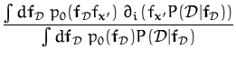
 +
+  P(
P( ln
ln