In the previous chapters learning algorithms for Gaussian processes
were derived. The presented algorithms had gradually increasing
complexity with the more complex algorithms embellished upon the
simpler ones. Specifically, if we include all training examples into
the
![]() set within the sparse online algorithm, then we obtain back
the online algorithm of Chapter 2. Similarly, using a
single sweep through the data for the sparse EP-algorithm of
Chapter 4 is equivalent to the sparse online algorithm
described in Chapter 3. Furthermore, when the
algorithms were defined, the likelihoods were left unspecified, it has
only been assumed that it is possible to evaluate - exactly or using
approximations - the averaged likelihood with respect to a
one-dimensional Gaussian measure which is needed to compute the update
coefficients for the online learning from Chapter 2.
set within the sparse online algorithm, then we obtain back
the online algorithm of Chapter 2. Similarly, using a
single sweep through the data for the sparse EP-algorithm of
Chapter 4 is equivalent to the sparse online algorithm
described in Chapter 3. Furthermore, when the
algorithms were defined, the likelihoods were left unspecified, it has
only been assumed that it is possible to evaluate - exactly or using
approximations - the averaged likelihood with respect to a
one-dimensional Gaussian measure which is needed to compute the update
coefficients for the online learning from Chapter 2.
For these reasons the experiments are grouped into a single chapter. This way more emphasis is given to the fact that sparse GP learning is applicable to a wide range of problems and at the same time the repetitions caused by presenting the same problem repeatedly for each algorithm are avoided. The aim of the experiments is to show the applicability of the sparse algorithms for various problems and the benefit of the approximation provided by sparsity. Thus, where it is possible, we present the results for the following cases:
Throughout the experiments two kernels are used: the polynomial
(eq. 138) and the radial basis function or RBF
(eq. 139) kernels:
where the d is the dimension of the inputs and we used it just for an approximate normalisation when using datasets of different dimensions. The kernel parameters are the order of the polynomial k and the length-scale lK for the first case and the width of the radial basis functions in the second case. The denominators in both cases include the normalisation constant d that makes the scaling of the kernels less dependent on the input dimensionality - independent if we assume that the data are normalised to unit variance. Both kernels are often used in practise. The polynomial kernels have a finite-dimensional feature space (discussed in Section 2.2) and are used for visualisation. The RBF kernels, having their origin in the area of radial basis function networks [7], have infinite-dimensional feature space; they are favourites in the kernel learning community.
The following sections detail the results of applying the sparse GP learning to different problems. Section 5.1 presents the results for regression, Section 5.2 for the classification. A non-parametric density estimation using the sparse GPs is sketched in Section 5.3. The final application considered is a data assimilation problem. In this case the problem is to infer a global model of wind fields using satellite observations. The GP approach to this problem and the possible benefits of sparsity are detailed in section 5.4.
|
Quadratic regression using Gaussian noise is analytically tractable [102] as has been detailed in previous chapters. The likelihood for a given example (x,y) in this case is
with
fx the GP marginal at the input location
x and
![]() the variance of the Gaussian noise (here supposed to be
known). It has been shown in Chapter 2 that online
learning applied to the Gaussian likelihood in
eq. (140) leads to an exact iterative computation of
the posterior process, expressed by its parameters
(
the variance of the Gaussian noise (here supposed to be
known). It has been shown in Chapter 2 that online
learning applied to the Gaussian likelihood in
eq. (140) leads to an exact iterative computation of
the posterior process, expressed by its parameters
(![]() ,C).
Using the kernel matrix
KN for all training data, the posterior
GP parameters are:
,C).
Using the kernel matrix
KN for all training data, the posterior
GP parameters are:
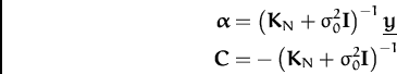 |
with
![]() the concatenation of all output values. The parameters
for the online recursions are
the concatenation of all output values. The parameters
for the online recursions are
q(t + 1) =  and r(t + 1) = - and r(t + 1) = -  |
where
kt + 1 = [K0(x1,xt + 1),..., K0(xt,xt + 1)]T
and
![]() = k* + kt + 1TCkt + 1 is the variance of
the GP marginal at
xt + 1.
= k* + kt + 1TCkt + 1 is the variance of
the GP marginal at
xt + 1.
The online algorithm from Chapter 2 uses
(![]() ,C) of the size of the training data. In
Chapter 3 it has been shown that this representation is
redundant: the dimensions of the GP parameters should not exceed the
dimension of the feature space. Introducing sparsity for the case of
regression keeps the GP representation non-redundant. To illustrate
this, first we consider the learning of the one-dimensional noisy
,C) of the size of the training data. In
Chapter 3 it has been shown that this representation is
redundant: the dimensions of the GP parameters should not exceed the
dimension of the feature space. Introducing sparsity for the case of
regression keeps the GP representation non-redundant. To illustrate
this, first we consider the learning of the one-dimensional noisy
![]() function
function
using the polynomial and the RBF kernels. In the experiments we
considered independent Gaussian noise with variance
![]() = 0.01.
First we considered the polynomial kernels from eq. (138).
These kernels, if the input space is one-dimensional, are particularly
simple: the dimension of the feature space associated with them is
k + 1. This means that the number of inputs in the
= 0.01.
First we considered the polynomial kernels from eq. (138).
These kernels, if the input space is one-dimensional, are particularly
simple: the dimension of the feature space associated with them is
k + 1. This means that the number of inputs in the
![]() set can never
be larger than k + 1. The KL-projection method from the sparse online
algorithm ensures this. The results from Fig. 5.1 show
that there are 6 examples in the
set can never
be larger than k + 1. The KL-projection method from the sparse online
algorithm ensures this. The results from Fig. 5.1 show
that there are 6 examples in the
![]() set, yet the GP contains
information about all data. When the RBF kernel is used, we see that
it provides a better approximation in this case, but the cost is that
there are twice as many elements in the
set, yet the GP contains
information about all data. When the RBF kernel is used, we see that
it provides a better approximation in this case, but the cost is that
there are twice as many elements in the
![]() set. The size of the
set. The size of the
![]() set has been set to 10 manually. For the
set has been set to 10 manually. For the
![]() function and RBF
kernels with
function and RBF
kernels with
![]() = 1,
= 1,
![]() set sizes larger than 12 were not
accepted: the score of each new input has been smaller than the
threshold for addition, which was set to 10-6 for numerical
stability.
set sizes larger than 12 were not
accepted: the score of each new input has been smaller than the
threshold for addition, which was set to 10-6 for numerical
stability.
![\includegraphics[]{fr_RBF_1_1_0.0001_250.eps}](img622.png)
|
The next example considered was the Friedman #1 dataset [23]. In this case the inputs are sampled uniformly from the 10-dimensional hypercube. The scalar output is obtained as
and the variables
x6,..., x10 do not affect the output, they
act as noise. Fig. 5.2 shows the test errors for
this dataset. From the clearly visible plateau as the
![]() set size
increases we conclude that the sparse online GP learning procedure
from Chapter 3, plotted with continuous lines, gives as
good solutions as the online learning that includes all examples to
the
set size
increases we conclude that the sparse online GP learning procedure
from Chapter 3, plotted with continuous lines, gives as
good solutions as the online learning that includes all examples to
the
![]() set. This suggests that the effective dimension of the data
in the feature space defined by the kernel is approximately 120 - 130
and there is no need to use more
set. This suggests that the effective dimension of the data
in the feature space defined by the kernel is approximately 120 - 130
and there is no need to use more
![]() s than this effective
dimensionality.
s than this effective
dimensionality.
The results of the GP learning were compared to those obtained by the
Support Vector regression (SVM) and the Relevance Vector machine (RVM)
as provided by [87]. The test error in the steady
region (i.e.
![]() set size > 120) for our algorithm was
set size > 120) for our algorithm was
![]() 2.4
which is smaller than those of the SVM (2.92) and RVM (2.80)
respectively. The number of parameters for GP algorithm, however, is
larger: it is quadratic in the size of the
2.4
which is smaller than those of the SVM (2.92) and RVM (2.80)
respectively. The number of parameters for GP algorithm, however, is
larger: it is quadratic in the size of the
![]() set whilst both the SVM
and the RVM algorithms have a linear scaling with respect to the size
of their ``support vectors'' (116 were used in the experiments) and
``relevance vectors'' (59 used) respectively.
set whilst both the SVM
and the RVM algorithms have a linear scaling with respect to the size
of their ``support vectors'' (116 were used in the experiments) and
``relevance vectors'' (59 used) respectively.
On the other hand, as discussed in Section 3.7, in their standard form both algorithms use the kernel matrix with respect to all data, this is not the case of the sparse EP/GP algorithm.
The sparse EP algorithm is applied in the second sweep through the
data. For cases when the size of the
![]() set is close enough to the
effective dimension of the data in the feature space, this second
sweep does not give any improvement. This is expected since for this
problem the posterior process is also a GP, no approximations are
involved in the online learning. As a result, in the region where the
set is close enough to the
effective dimension of the data in the feature space, this second
sweep does not give any improvement. This is expected since for this
problem the posterior process is also a GP, no approximations are
involved in the online learning. As a result, in the region where the
![]() set sizes exceed this effective dimension, the KL-projection in
the sparse online algorithm is just a rewriting of the feature space
image of the new input as a combination of inputs from the
set sizes exceed this effective dimension, the KL-projection in
the sparse online algorithm is just a rewriting of the feature space
image of the new input as a combination of inputs from the
![]() set,
and the length of the residual is practically zero. If we are not
close to the limit region, then the EP corrections improve on the
performance of the algorithm, as it is the case for the small
set,
and the length of the residual is practically zero. If we are not
close to the limit region, then the EP corrections improve on the
performance of the algorithm, as it is the case for the small
![]() set
sizes in Fig. 5.2. This improvement is not
significant for regression, the improvements are within the
empirical error bars, as it is also shown for the next application:
the Boston housing dataset.
set
sizes in Fig. 5.2. This improvement is not
significant for regression, the improvements are within the
empirical error bars, as it is also shown for the next application:
the Boston housing dataset.
The Boston housing dataset is a real dataset with 506 data, each
having 13 dimensions and a single output. The 13 inputs describe
different characteristics of houses and the task is to predict their
price.7In the experiments the dataset has been split into training and test
sets of sizes 481/25 and we used 100 random splits for all
![]() set
sizes and the results are shown in Fig. 5.3. If
different
set
sizes and the results are shown in Fig. 5.3. If
different
![]() set sizes are compared, we see that there is no
improvement after a certain
set sizes are compared, we see that there is no
improvement after a certain
![]() set size.
set size.
Two series of experiments were considered by using the same dataset
without pre-processing (sub-figure a), or normalising it to zero mean
and unit variance (subfigure b). The results have been compared with
the SVM and RVM methods, which had squared errors approximately
8 [87], we conclude that the performance of the
sparse GP algorithm is comparable to these other kernel algorithms.
We need to mention however that, the setting of the hyper-parameters
![]() and
and
![]() was made on a trial-and error, we did
not use cross-validation or other hyper-parameter selection method,
the aim of the thesis is to show the applicability of the sparse GP
framework to real-world problems.
was made on a trial-and error, we did
not use cross-validation or other hyper-parameter selection method,
the aim of the thesis is to show the applicability of the sparse GP
framework to real-world problems.
|
We see that if the size of the
![]() set is large enough, the
expectation-propagation algorithm does not improve on the performance
of the sparse online algorithm. Improvements when the data is
re-used are visible only if the
set is large enough, the
expectation-propagation algorithm does not improve on the performance
of the sparse online algorithm. Improvements when the data is
re-used are visible only if the
![]() set is small. This improvement is
not visible when learning the unnormalised Boston dataset.
set is small. This improvement is
not visible when learning the unnormalised Boston dataset.
The main message from this section is that using sparsity in the GPs does not lead to significant decays in the performance of the algorithm. However, the differences between the sub-plots in Fig. 5.3 emphasises the necessity of developing methods to adjust the hyper-parameters. In the next section we present examples where the EP-algorithm improves on the results of the sparse online learning: classification using GPs.
A nontrivial application of the online GPs is the classification
problem: the posterior process is non-Gaussian and we need to perform
approximations to obtain a GP from it. We use the probit
model [49] where a binary value
y ![]() { - 1, 1} is assigned to
an input
x
{ - 1, 1} is assigned to
an input
x ![]()
![]() m with the data likelihood
m with the data likelihood
where ![]() is the noise variance and
is the noise variance and
![]() is the cumulative
Gaussian distribution:
is the cumulative
Gaussian distribution:
The shape of this likelihood resembles a sigmoidal, the main benefit of this choice is that its average with respect to a Gaussian measure is computable. We can compute the predictive distribution at a new example x:
where
![]() fx
fx![]() = kxT
= kxT![]() is the mean of the GP at
x and
is the mean of the GP at
x and
![]() =
= ![]() + k*x + kxTCkx. It is the
predictive distribution of the new data, that is the Gaussian average
of an other Gaussian. The result is obtained by changing the order of
integrands in the Bayesian predictive distribution
eq. (143) and back-substituting the definition of the
error function.
+ k*x + kxTCkx. It is the
predictive distribution of the new data, that is the Gaussian average
of an other Gaussian. The result is obtained by changing the order of
integrands in the Bayesian predictive distribution
eq. (143) and back-substituting the definition of the
error function.
Based on eq. (53), for a given input-output pair (x, y) the update coefficients q(t + 1) and r(t + 1) are computed by differentiating the logarithm of the averaged likelihood from eq. (145) with respect to the mean at xt + 1 [17]:
with
![]() evaluated at
z =
evaluated at
z =  and
and
![]() and
and
![]() are the
first and second derivatives at z.
are the
first and second derivatives at z.
|
The algorithm for classification was first tested with two small
datasets. These small-sized data allowed us to benchmark the sparse
EP algorithm against the full EP algorithm presented in
Chapter 4. The first dataset is the Crab
dataset [66] 8. This dataset has
6-dimensional inputs, measuring different characteristics of the
Leptograpsus crabs and the task is to predict their gender. There are
200 examples split into 80/120 training/test sets. In the
experiments we used the splits given in [99] and we
used the RBF kernels to obtain the results shown
Fig 5.4.a (the polynomial kernels gave slightly larger
test errors). As for the regression case, we see the long plateau for
the sparse online algorithm (the thick continuous line labeled ``1
sweep'') when the
![]() set size increases. We also see that the online
and the sparse online learning algorithms have a relatively large
variation in their performance, as shown by the error-bars.
set size increases. We also see that the online
and the sparse online learning algorithms have a relatively large
variation in their performance, as shown by the error-bars.
The result of applying the full EP algorithm of [46] can
be seen when all 80 basis vectors are included into the
![]() set in
Fig. 5.4.a. We see that the average performance of the
algorithm improved when a second and a third iteration through the
data is made. Apart from the decrease in the test error, by the end of
the third iteration the fluctuations caused by the ordering of the
data also vanished.
set in
Fig. 5.4.a. We see that the average performance of the
algorithm improved when a second and a third iteration through the
data is made. Apart from the decrease in the test error, by the end of
the third iteration the fluctuations caused by the ordering of the
data also vanished.
As the dashed line from Fig. 5.4.a shows, if the size of
the
![]() set is larger than 20, the sparse EP algorithm has the
same behaviour as the full EP, reaching a test error of 2.5%,
meaning 3 misclassified examples from the test set. Interestingly
this small test error is reached even if more than 80% of the
inputs were removed,in showing the benefit of combining the EP
algorithm with the sparse online GP. The performance of the algorithm
is in the range of the results of other the state-of-the-art methods:
3 errors with the TAP mean field method, 2 using the naive mean
field method [58], 3 errors when applying the
projection pursuit regression method [66].
set is larger than 20, the sparse EP algorithm has the
same behaviour as the full EP, reaching a test error of 2.5%,
meaning 3 misclassified examples from the test set. Interestingly
this small test error is reached even if more than 80% of the
inputs were removed,in showing the benefit of combining the EP
algorithm with the sparse online GP. The performance of the algorithm
is in the range of the results of other the state-of-the-art methods:
3 errors with the TAP mean field method, 2 using the naive mean
field method [58], 3 errors when applying the
projection pursuit regression method [66].
Fig. 5.4.b shows a cross-section of the simulations for
![]() . The top sub-figure plots the average test and training
errors with the empirical deviations of the errors (the dashed lines).
The additional computational cost of the algorithm, compared with the
sparse online method, is the update of the projection matrix
P,
requiring
. The top sub-figure plots the average test and training
errors with the empirical deviations of the errors (the dashed lines).
The additional computational cost of the algorithm, compared with the
sparse online method, is the update of the projection matrix
P,
requiring
![]() (Nd ) operations. This update is needed only if we
are replacing an element from the
(Nd ) operations. This update is needed only if we
are replacing an element from the
![]() set. The bottom part of
Fig. 5.4.b shows the average number of changes in the
set. The bottom part of
Fig. 5.4.b shows the average number of changes in the
![]() set. Although there are no changes in the test or the training
errors after the second iteration, the costly modification of the
set. Although there are no changes in the test or the training
errors after the second iteration, the costly modification of the
![]() set is still performed relatively often, suggesting that the changes
in the
set is still performed relatively often, suggesting that the changes
in the
![]() set after this stage are not important. This suggests that
for larger datasets we could employ different strategies for speeding
up the algorithm. One simple suggestion is to fix the elements in the
set after this stage are not important. This suggests that
for larger datasets we could employ different strategies for speeding
up the algorithm. One simple suggestion is to fix the elements in the
![]() set after the second iteration and to perform the sparse EP
algorithm by projecting the data to the subspace of the
set after the second iteration and to perform the sparse EP
algorithm by projecting the data to the subspace of the
![]() elements
in the subsequent iterations. The later stage of the algorithm would
be as fast as the sparse online algorithm since the storage of the
matrix
P is not required. A second strategy would be to
choose the kernel parameters and the size of the
elements
in the subsequent iterations. The later stage of the algorithm would
be as fast as the sparse online algorithm since the storage of the
matrix
P is not required. A second strategy would be to
choose the kernel parameters and the size of the
![]() set such that the
number of replacements is low, the given number of basis vectors
representing all training inputs, this is possible using appropriate
pre-processing or adapting the model parameters accordingly.
set such that the
number of replacements is low, the given number of basis vectors
representing all training inputs, this is possible using appropriate
pre-processing or adapting the model parameters accordingly.
The selection of the parameters for the RBF kernel is not discussed.
When running the different experiments we observed that the size of
the
![]() set and the optimal kernel parameters are strongly related,
making the model selection issue an important future research topic.
set and the optimal kernel parameters are strongly related,
making the model selection issue an important future research topic.
|
A second experiment for classification used the sonar
data [29].9. This dataset
has originally been used to test classification performance using
neural networks. It consists of 208 measurements of sonar signals
bounced back from a cylinder made of metal or rock, each having 60
components. In the experiments we used the same split of the data as
has been used by [29]. The data was preprocessed
to unit variance in all components and we used RBF kernels with
variance
![]() = 0.25, with noise
= 0.25, with noise
![]() = 0.0001. The results
for different
= 0.0001. The results
for different
![]() set sizes are presented in Fig. 5.5.
We can again see a plateau of almost constant test error performance
starting at 70. Contrary to the case of the Crab dataset, this
plateau is not as clear as in Fig. 5.5; a drop in the
test error is visible at the upper limit of the
set sizes are presented in Fig. 5.5.
We can again see a plateau of almost constant test error performance
starting at 70. Contrary to the case of the Crab dataset, this
plateau is not as clear as in Fig. 5.5; a drop in the
test error is visible at the upper limit of the
![]() set sizes. The
difference might be due to the higher dimensionality of the data: 60
as opposed to 6 whilst the sizes of the training sets are
comparable.
set sizes. The
difference might be due to the higher dimensionality of the data: 60
as opposed to 6 whilst the sizes of the training sets are
comparable.
For comparison with other algorithms we used the results as reported
in [58]. The test errors of the naive mean field
algorithm and the TAP mean field algorithm were 7.7, this being the
closest to the result of the EP algorithm which was 6.7. It is also
important that the EP test error at
![]() , i.e. when using
almost all training data, becomes independent of the order of the
presentation, the error bars vanish.
, i.e. when using
almost all training data, becomes independent of the order of the
presentation, the error bars vanish.
However, using only a half the training data in the
![]() set, the
performance of the sparse EP algorithm is
8.9±0.9%, still as good
as the SVM or the best performing two-layered neural network both of
which are reported to have 9.6% as test
errors [66,58].
set, the
performance of the sparse EP algorithm is
8.9±0.9%, still as good
as the SVM or the best performing two-layered neural network both of
which are reported to have 9.6% as test
errors [66,58].
A third dataset which we have used in tests is the USPS dataset of
gray-scale handwritten digit images of size
16×16. The dataset
consists of 7291 training and 2007 test
patterns.10 In the first experiment we
studied the problem of classifying the digit 4 against all other
digits. Fig. 5.6.a plots the test errors of the
algorithm for different
![]() set sizes and fixed values of
hyper-parameter
set sizes and fixed values of
hyper-parameter
![]() = 0.5.
= 0.5.
|
The USPS dataset has frequently been used to test the performance of kernel-based classification algorithms. We mention the kernel PCA method of [73], the Nyström method of [101] and the application of the kernel matching pursuit algorithm [94], all discussed in detail in Section 3.7.
The Nyström approach considers a subset of the training data onto
which the inputs are projected, thus it is similar to the sparse GP
algorithm. This approximation proved to provide good results if the
size of the subset was as low as 256. The mean of the test error
for this case was
![]() 1.7% [101], thus the
results from Fig. 5.6.a are in the same range.
1.7% [101], thus the
results from Fig. 5.6.a are in the same range.
The PCA reduced-set method of [73] and the kernel matching pursuit algorithms give very similar results for the USPS dataset, their result sometimes is as low as 1.4%. By performing additional model selection the results of the sparse GP/EP algorithms could be improved, our aim for these experiments was to prove that the algorithm produces similar results to other sparse algorithms in the family of kernel methods.
|
The sparse EP algorithm was also tested on the more realistic problem
of classifying all ten digits simultaneously. The ability to compute
Bayesian predictive probabilities is absolutely essential in this
case. We have trained 10 classifiers on the ten binary classification
problems of separating a single digit from the rest. An unseen input
was assigned to the class with the highest predictive probability
given by eq. (145). Fig. 5.6.b
summarises the results for the multi-class case for different
![]() set
sizes and RBF kernels (with the external noise variance
set
sizes and RBF kernels (with the external noise variance
![]() = 0).
= 0).
To reduce the computational cost we used the same set for all individual classifiers (only a single inverse of the Gram matrix was needed and also the storage cost is smaller). This made the implementation of deleting a basis vector for the multi-class case less straightforward: for each input and each basis vector there are 10 individual scores. We implemented a ``minimax'' deletion rule: whenever a deletion was needed, the basis vector having the smallest maximum value among the 10 classifier problems was deleted, i.e. the index l of the deleted input was
The results of the combined classification for 100 and 350
![]() s is shown in Fig. 5.6.b The sparse online
algorithm gave us a test error of 5.4% and the sparse EP refinement
further improved the results to 5.15%. It is important that in
obtaining the test errors we used the same 350 basis vectors
for all binary classifiers. This is important, especially if we are
to make predictions for an unknown digit. If we use the SVM approach
and compute the 10 binary predictions, then we need to evaluate the
kernel 2560 times, opposed to the 350 evaluation for the basis
vector case. The results from Fig. 5.6.b are also close
to the batch performance reported in [73]. The
combination of the 10 independent classifiers obtained using kernel
PCA attained a test error of 4.4%.
s is shown in Fig. 5.6.b The sparse online
algorithm gave us a test error of 5.4% and the sparse EP refinement
further improved the results to 5.15%. It is important that in
obtaining the test errors we used the same 350 basis vectors
for all binary classifiers. This is important, especially if we are
to make predictions for an unknown digit. If we use the SVM approach
and compute the 10 binary predictions, then we need to evaluate the
kernel 2560 times, opposed to the 350 evaluation for the basis
vector case. The results from Fig. 5.6.b are also close
to the batch performance reported in [73]. The
combination of the 10 independent classifiers obtained using kernel
PCA attained a test error of 4.4%.
The benefit of the probabilistic treatment of the classification is that we can reject some of the data: the ones for which the probability of belonging to any of the classes is smaller then a predefined threshold. In Fig. 5.7 we plot the test errors and the rejected inputs for different threshold values.
An immediate extension of the sparse classification algorithms would be to extend them for the case of active learning [75,9] described in Section 3.8.1. It is expected that this extension, at the cost of searching among the training data, would improve the convergence of the algorithm.
To sum up, in the classification case, contrary to regression, we had a significant improvement when using the sparse EP algorithm. The improvement was more accentuated in the low-dimensional case. The important benefit of the EP algorithm for classification was to make the results (almost) independent of the order of presentation, as seen in the figures showing the performance of the EP algorithm.
Density estimation is an unsupervised learning problem: we have a set
of p-dimensional data
![]() = {xi}i = 1N and our goal is
to approximate the density that generated the data. This is an
ill-posed problem, the weighted sum of delta-peaks being an extreme of
the possible solutions [93]. In one-dimensional case a
common density estimation method is the histogram, and the
Parzen-windowing technique can be thought as an extension of the
histogram method to the multi-dimensional case. In this case the
kernel is
K0(x,x) = h(|x - x
= {xi}i = 1N and our goal is
to approximate the density that generated the data. This is an
ill-posed problem, the weighted sum of delta-peaks being an extreme of
the possible solutions [93]. In one-dimensional case a
common density estimation method is the histogram, and the
Parzen-windowing technique can be thought as an extension of the
histogram method to the multi-dimensional case. In this case the
kernel is
K0(x,x) = h(|x - x![]() |2) with the function h
chosen such that
|2) with the function h
chosen such that
![]() dxK0(x,x
dxK0(x,x![]() ) = 1 for all
x
) = 1 for all
x![]() . The
Parzen density estimate,based on K0, is written [21]:
. The
Parzen density estimate,based on K0, is written [21]:
where the prefactor 1/N to the sum can be thought of as a coefficient
![]() that weights the contribution of each input to the inferred
distribution. The difficulty in using this model, as with other
non-parametric techniques, is that it cannot be used for large data
sizes. Even if there is no cost to compute
that weights the contribution of each input to the inferred
distribution. The difficulty in using this model, as with other
non-parametric techniques, is that it cannot be used for large data
sizes. Even if there is no cost to compute ![]() , the storage of
each training point and the summation is infeasible, raising the need
for simplifications.
, the storage of
each training point and the summation is infeasible, raising the need
for simplifications.
Recent studies addressed this problem using other kernel methods,
based on the idea of Support Vector Machines.
[97] used SVMs for density estimation. Instead of
using the fixed set of coefficients
![]() = 1/N, they allowed these
coefficients to vary. An additional degree of freedom to the problem
was added by allowing kernels with varying shapes to be included in
eq. (148). The increase in complexity was
compensated with corresponding regularisation penalties. The result
was a sparse representation of the density function with only a few
coefficients having nonzero parameters. This made the computation of
the inferred density function faster, but to obtain the sparse set of
solutions, a linear system using all data points had to be solved.
= 1/N, they allowed these
coefficients to vary. An additional degree of freedom to the problem
was added by allowing kernels with varying shapes to be included in
eq. (148). The increase in complexity was
compensated with corresponding regularisation penalties. The result
was a sparse representation of the density function with only a few
coefficients having nonzero parameters. This made the computation of
the inferred density function faster, but to obtain the sparse set of
solutions, a linear system using all data points had to be solved.
A different method was the use of orthogonal series expansion of kernels used for Parzen density estimation in eq. (148), proposed by [28]. This mapped the problem into a feature space determined by the orthogonal expansion. The sparsity is achieved by using kernel PCA [70] or the Nyström method for kernel machines [101]. The study presented empirical comparisons between the performance of the kernel PCA density estimation and the original Parzen method, showing that a significant reduction of the components from the sum was possible without decay in the performance of the estimation.
In this section we apply the sparse GPs and the EP algorithm to obtain a Bayesian approach to density estimation. We use a random function f to model the distribution and the prior over the function f regularises the density estimation problem.
The prior over the functions is a GP and next we define the likelihood. A basic requirement for a density function is to be non-negative and normalised, thus we consider the likelihood model:
with fx a random function drawn from the prior process and h(x| f ) is the density at the input x. An important difference from the previous cases is that the likelihood for a single output is conditioned on the whole process. We assume a compact domain for the inputs, this makes the normalising integral well defined. Another possibility would be to assume a generic prior density for the inputs to replace the constraint on the input domain, however this is future work.
In contrast to the previous applications of the sequential GP learning
presented in this Chapter, this ``likelihood'' is not local: the
density at a point is dependent on all other values of f, the
realisation of the random process. This density model has been
studied in [34] and [69] and other likelihoods
for density estimation have also been considered like
p(x| f ) ![]() exp(- fx) by [50], but these
earlier studies were concerned with finding the maximum a-posteriori
value of the process.
exp(- fx) by [50], but these
earlier studies were concerned with finding the maximum a-posteriori
value of the process.
We are using eq. (149) to represent the density, making the inference of the unknown probability distribution equivalent to learning the underlying process. We write the posterior for this process as
where again, due to the denominator, we need to take into account all possible realisations of the function f, i.e. we have a functional integral.
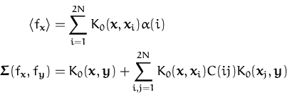
As usual, we are interested in the predictive distribution of the density, which is given by eq. (149) where fx is the marginal of the posterior GP at x. We obtain a random variable for the density at x. We compute the mean of this random value, and have the prediction for the density function:
with the normalising constant Z defined in eq (150).
The normalisation in the previous equations makes the density model intractable. Essentially, it prevents the solutions from being expressible using the representer theorem of [40] or the representation lemma from Chapter 2. Next we transform the posterior into a form that makes the representation lemma applicable for the density estimation problem. For this we observe that the normalising term is independent of the input set and of the location at which the distribution is examined. To apply the parametrisation lemma, we include the normalising term into the prior to obtain a new prior for f. For this we consider the Gamma-distribution
where the integral with respect to
fz is considered fixed. We
can rewrite the predicted density by adding ![]() to the set of
model parameters:
to the set of
model parameters:
where an expectation over a new Gaussian prior has been introduced.
The new GP is obtained by multiplying the initial GP with the
exponential from eq. (152) and Z![]() is the
normalisation corresponding to new ``effective GP''.
is the
normalisation corresponding to new ``effective GP''.
Next we derive the covariance of this ``effective GP''. For this we
use the decomposition of the kernels K0 using an orthonormal set of
eigen-functions
![]() (x). For this set of functions we have
(x). For this set of functions we have
such that
K0(x,x![]() ) =
) = ![]()
![]()
![]() (x)
(x)![]() (x
(x![]() ),
the details of the different mappings into the feature space were
presented in Section 2.1. We used
),
the details of the different mappings into the feature space were
presented in Section 2.1. We used
![]() to denote
the eigenvalues in order to avoid possible confusions that would
result from double meaning of the parameter
to denote
the eigenvalues in order to avoid possible confusions that would
result from double meaning of the parameter ![]() .
.
The decomposition of the kernel leads to the projection function from the input into the feature space:
and we can write the random function
fx = f (x) = ![]() T
T![]() (x) where
(x) where
![]() = [
= [![]() ,
,![]() ,...]T is the vector of
random variables in the feature space and we used the vector
notations.
,...]T is the vector of
random variables in the feature space and we used the vector
notations.
We want to express the normalisation integral using the feature space.
The orthonormality of
![]() (x) from eq. (154)
implies that
(x) from eq. (154)
implies that
where
L is a diagonal matrix with
![]() on the diagonal.
The modified Gaussian distribution of the feature space
variables is be written as:
on the diagonal.
The modified Gaussian distribution of the feature space
variables is be written as:
and this change implies that the kernel for the ``effective GP'' is
where the initial projection into the feature space and the modified
distribution of the random variables in that feature space was used.
The final form of the GP kernel is found by observing that
K![]() has the same eigenfunctions but the eigenvalues are
(
has the same eigenfunctions but the eigenvalues are
(![]() +
+ ![]() )-1, thus
)-1, thus
As a result of previous transformations, the normalising term from the
likelihood was eliminated by adding ![]() to the model
parameters.11 This simplifies the
likelihood, but for each
to the model
parameters.11 This simplifies the
likelihood, but for each ![]() we have different GP kernel, and to
find the most probable density, we have to integrate over
we have different GP kernel, and to
find the most probable density, we have to integrate over ![]() ,
this is not feasible in practise.
,
this is not feasible in practise.
Our aim is to approximate the posterior
p(x|![]() ) from
eq. (153) with a GP in such a way that we are
able to apply the representation lemma from Chapter 2.
For this we first eliminate the integral with respect to
) from
eq. (153) with a GP in such a way that we are
able to apply the representation lemma from Chapter 2.
For this we first eliminate the integral with respect to ![]() and
then approximate the kernel in the effective Gaussian from
eq. (159).
and
then approximate the kernel in the effective Gaussian from
eq. (159).
The integral over ![]() is eliminated using a maximum a-posteriori
(MAP)approximation.
We compute
is eliminated using a maximum a-posteriori
(MAP)approximation.
We compute
![]() that maximises the log-integrand in
eq. (153). Setting its derivative to zero
leads to
that maximises the log-integrand in
eq. (153). Setting its derivative to zero
leads to
We replace the integral over ![]() with its value at
with its value at ![]() and to simplify the notations, in the following we ignore the
subscript. The predictive density becomes
and to simplify the notations, in the following we ignore the
subscript. The predictive density becomes
Using this approximation to the predictive density, we can employ the parametrisation lemma and the sequential algorithms, as in the previous cases, to infer a posterior process. We observe that in the numerator of eq. (161) we have a product of single data likelihoods fi2, this time without the normalisation as in in eq. (149), and the denominator is the normalisation required by the posterior.
The application of the EP algorithm for this modified GP becomes
straightforward. For a fixed ![]() we use the ``effective GP''
from eq. (159) as the prior process. We iterate
the EP learning from Chapter 4 and obtain a posterior
process with the data-dependent parameters
(
we use the ``effective GP''
from eq. (159) as the prior process. We iterate
the EP learning from Chapter 4 and obtain a posterior
process with the data-dependent parameters
(![]() ,C). The
parameters also depend on
,C). The
parameters also depend on ![]() , thus the complete GP will be
characterised with the triplet, which we denote
, thus the complete GP will be
characterised with the triplet, which we denote
![]() . Changing the GP parameters changes
. Changing the GP parameters changes
![]() , thus at the end of each EP iteration we recompute
, thus at the end of each EP iteration we recompute
![]() , this time fixing
(
, this time fixing
(![]() ,C). Using the posterior GP
in eq. (160), the re-estimation equation for
,C). Using the posterior GP
in eq. (160), the re-estimation equation for
![]() is
is
and we can iterate the EP algorithm using the new GP.
The problem is finding the kernel that corresponds to the ``effective
![]() ''. Finding
''. Finding
![]() or general kernels requires
the eigenvalues of the kernel, or an inverse operation in the feature
space. This is seldom tractable analytically, we mention different
approaches to address this inversion applied to density estimation.
One is to find the inverse operator by numerically solving
eq. (159), employed by
[50], although this is extremely time-consuming.
A different solution is to use the operator product expansion
in [69]:
or general kernels requires
the eigenvalues of the kernel, or an inverse operation in the feature
space. This is seldom tractable analytically, we mention different
approaches to address this inversion applied to density estimation.
One is to find the inverse operator by numerically solving
eq. (159), employed by
[50], although this is extremely time-consuming.
A different solution is to use the operator product expansion
in [69]:
to obtain
![]() . Apart from being, again, computationally
expensive, this expansion is unstable for large
. Apart from being, again, computationally
expensive, this expansion is unstable for large ![]() values.
values.
A simplification of the inversion problem is to choose the prior
kernels in a convenient fashion such as to provide tractable models.
A choice for the operator for one-dimensional inputs was
l2![]() , used by [34] to estimate densities. This
operator implies the Ornstein-Uhlenbeck kernels for
, used by [34] to estimate densities. This
operator implies the Ornstein-Uhlenbeck kernels for
![]() :
:
Since ![]() increases with the size of the data, the resulting
density function, being a weighted sum of kernel functions, will be
very rough.
increases with the size of the data, the resulting
density function, being a weighted sum of kernel functions, will be
very rough.
A different simplification is obtained if we choose the prior operator
![]() such that
such that
![]() . This means that all
eigenvalues are equal
. This means that all
eigenvalues are equal
![]() = 1 and the inverse from
eq. (159) simplifies to
= 1 and the inverse from
eq. (159) simplifies to
 |
If we use one-dimensional inputs from the interval [0, 1] and consider a finite-dimensional function space with elements
where an, bn, and c0 are sampled randomly from a Gaussian
distribution with zero mean and unit variance. It is easy to check
that the 2k0 + 1 functions from eq. (166) are
orthonormal. Since we know that the eigenvalues are all equal to 1,
this kernel is idempotent
![]() , thus the inversion is
reduced to a division with a constant. We compute the kernel that
generates these functions:
, thus the inversion is
reduced to a division with a constant. We compute the kernel that
generates these functions:
where the average is taken over the set of random variables (an, bn) and c0. Fig. 5.8 shows the kernel for k0 = 5 and the experiments were performed using this kernel.
Next we have to solve eq. (162) to find
![]() . We assume that we are at the end of the first iteration,
when
. We assume that we are at the end of the first iteration,
when ![]() = 0 on the RHS. In this case eq. (162)
simplifies and we obtain
= 0 on the RHS. In this case eq. (162)
simplifies and we obtain
where we used the reproducing property of the kernel and expressed the
predictive mean and covariance at
x using the representation
given by the parameters
(![]() ,C):
,C):
with p the size of the
![]() set.
set.
To apply online learning, we have to compute the average over the
likelihood. Assuming that we have an approximation to the
![]() , we need to compute the average with respect to
, we need to compute the average with respect to
![]() , the marginal GP at
xt + 1. The
averaged likelihood is
, the marginal GP at
xt + 1. The
averaged likelihood is
![]() ft + 12
ft + 12![]() =
= ![]() +
+ ![]() , and the update coefficients are the first and the
second derivatives of the log-average (from
eq. 53)
, and the update coefficients are the first and the
second derivatives of the log-average (from
eq. 53)
q(t + 1) =  and r(t + 1) = and r(t + 1) = 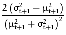 . . |
We used an artificial dataset generated from a mixture of two
Gaussians, plotted with dashed lines in Fig. 5.9.a.
The size of the data set in simulations was 500 and we used k0 = 5
for the kernel parameter. The learning algorithm was the sparse EP
learning as presented in Chapter 4 with the
![]() set size
not fixed in advance. We allowed the
set size
not fixed in advance. We allowed the
![]() set to be updated each time
the score of a new input was above the predefined threshold, since for
this toy example, the dimension of the feature space is 2k0 + 1. The
KL-criterion prevents a the
set to be updated each time
the score of a new input was above the predefined threshold, since for
this toy example, the dimension of the feature space is 2k0 + 1. The
KL-criterion prevents a the
![]() set from becoming larger than the
dimension of the feature space, thus there is no need for pruning the
GPs.
set from becoming larger than the
dimension of the feature space, thus there is no need for pruning the
GPs.
|
To summarise, this section outlined a possibility to use GPs for
density estimation. The applicability of the model in its present
form is restricted, we gave results only for one-dimensional density
modelling. The essential step in obtaining this density model was the
transformation of the problem such that the iterative GP algorithms
were made applicable. This was achieved by choosing special kernels
corresponding to operators satisfying
![]() ,
condition needed to simplify the operator inversion
eq. (163). Further simulations could be made
using higher-dimensional inputs for which these kernels are also
computable, however we believe that the basic properties of this model
are highlighted using this toy example.
,
condition needed to simplify the operator inversion
eq. (163). Further simulations could be made
using higher-dimensional inputs for which these kernels are also
computable, however we believe that the basic properties of this model
are highlighted using this toy example.
The GP density estimation has certain benefits: contrary to mixture
density modelling, it does not need a predefined number of mixture
components. The corresponding entity, the
![]() set size in this model
is determined automatically, based on the data and the hyper-parameters
of the model. An other advantage is computational: we do not need to
store the full kernel matrix, opposite to the case of
SVMs [97] or the application of the kernel
PCA [28]. A drawback of the model, apart from the need
to find the proper hyper-parameters, is that the convergence time can
be long, as it is shown in Fig. 5.9.b. More
theoretical study is required for speeding up the convergence and
making the model less dependent on the prior assumptions.
set size in this model
is determined automatically, based on the data and the hyper-parameters
of the model. An other advantage is computational: we do not need to
store the full kernel matrix, opposite to the case of
SVMs [97] or the application of the kernel
PCA [28]. A drawback of the model, apart from the need
to find the proper hyper-parameters, is that the convergence time can
be long, as it is shown in Fig. 5.9.b. More
theoretical study is required for speeding up the convergence and
making the model less dependent on the prior assumptions.
In this section we consider the problem of data assimilation where we aim to build a global model based on spatially distributed observations [15]. GPs are well suited for this type of application, providing us with a convenient way of relating different observations.
The data was collected from the ERS-2 satellite [51] where the aim is to obtain an estimate of the wind fields which the scatterometer indirectly measures using radar backscatter from the ocean surface. There are significant difficulties in obtaining the wind direction from the scatterometer data, the first being the presence of symmetries in the model: wind fields that have opposite directions result in almost equal measurements [22,48], making the wind field retrieval a complex problem with multiple solutions. Added the inherent noise in the observations increases the difficulty we face in the retrieval process.
Current methods of transforming the observed values (scatterometer data, denoted as a vector si at a given spatial location xi) into wind fields can be split into two phases: local wind vector retrieval and ambiguity removal [84] where one of the local solutions is selected as the true wind vector. Ambiguity removal often uses external information, such as a Numerical Weather Prediction (NWP) forecast of the expected wind field at the time of the scatterometer observations.
[47] have recently proposed a Bayesian framework for wind field retrieval combining a vector Gaussian process prior model with local forward (wind field to scatterometer) or inverse models. The backscatter is measured over 50×50 km cells over the ocean and the number of observations acquired can be several thousand, making GPs hardly applicable to this problem.
In this section we build a sparse GP that scales down the computational needs of the conventional GPs, this application was presented in [16].
![\includegraphics[]{MDN.eps}](img758.png) |
We use a mixture density network (MDN) [4] to model the conditional dependence of the local wind vector zi = (ui, vi) on the local scatterometer observations si:
where
![]() is the union of the MDN parameters: for each
observation at location
xi we have the set weightings
is the union of the MDN parameters: for each
observation at location
xi we have the set weightings
![]() for the
local Gaussians
for the
local Gaussians
![]() (cij,
(cij,![]() ) where
cij is the
mean and
) where
cij is the
mean and
![]() is the variance. The parameters of the MDN
are determined using an independent training set [22]
and are considered known in this section.
is the variance. The parameters of the MDN
are determined using an independent training set [22]
and are considered known in this section.
The MDN with four Gaussian component densities captures the ambiguity of the inverse problem. An example of a 10×10 field produced by the MDN is shown in Fig 5.10. We see that for the majority of the spatial locations we have symmetries in the MDN solution: the model prefers a speed, but the orientation of the resulting wind-vector is uncertain.
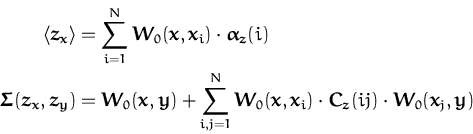
In order to have a global model from the N wind vectors obtained by local inversion using eq. (169), we combine them with a zero-mean vector GP [13,47]:
| q( |
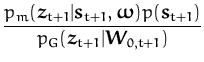
and instead of using the direct likelihood p(si|zi), we transform it using Bayes theorem again to obtain:
where
![]() = [z1,...,zN]T is the concatenation of the local
wind field components
zi. These components are random variables
corresponding to a spatial location
xi. These locations specify
the prior covariance matrix for the vector
= [z1,...,zN]T is the concatenation of the local
wind field components
zi. These components are random variables
corresponding to a spatial location
xi. These locations specify
the prior covariance matrix for the vector
![]() , given by
W0 = {W0(xi,xj)}ij = 1N. The two-dimensional
Gaussian p0 is the prior GP marginalised at zi, with zero-mean
and covariance
W0i. The prior GP was tuned carefully to
represent features seen in real wind fields.
, given by
W0 = {W0(xi,xj)}ij = 1N. The two-dimensional
Gaussian p0 is the prior GP marginalised at zi, with zero-mean
and covariance
W0i. The prior GP was tuned carefully to
represent features seen in real wind fields.
Since all quantities involved are Gaussians, we could, in
principle, compute the resulting probabilities analytically, but
this computation is practically intractable: the number of
mixture elements from
q(![]() ) is 4N which is extremely high even
for moderate values of N. Instead, we will apply the online
approximation to have a jointly Gaussian approximation to the
posterior at all data points.
) is 4N which is extremely high even
for moderate values of N. Instead, we will apply the online
approximation to have a jointly Gaussian approximation to the
posterior at all data points.
Due to the vector GP, the kernel function
W0(x,y) is a
2×2 matrix, specifying the pairwise cross-correlation between
wind field components at different spatial positions. The
representation of the posterior GP thus requires vector quantities:
the marginal of the vector GP at a spatial location
x has a
bivariate Gaussian distribution with mean and covariance function of
the vectors
zx ![]()
![]() 2 represented as
2 represented as
where
![]() z(1),
z(1),![]() z(2),...,
z(2),...,![]() z(N) and
{Cz(ij)}i, j = 1, N of the vector GP. Since this form is not
convenient, we represent (for numerical convenience) the vectorial
process by a scalar process with twice the number of observations,
i.e. we set
z(N) and
{Cz(ij)}i, j = 1, N of the vector GP. Since this form is not
convenient, we represent (for numerical convenience) the vectorial
process by a scalar process with twice the number of observations,
i.e. we set
where K0(x,y) is a scalar valued function which we are going to use purely for notation. Since we are dealing with vector quantities, we will never have to evaluate the individual matrix elements. K0 serves us just for re-arranging the GP parameters in a more convenient form. By ignoring the superscripts v and u, we can write
where
![]() = [
= [![]() ,...,
,...,![]() ]T and
C = {C(ij)}i, j = 1,..., 2N are rearrangements of the parameters
from eq. (171).
]T and
C = {C(ij)}i, j = 1,..., 2N are rearrangements of the parameters
from eq. (171).
For a new observation st + 1 we have a a local "likelihood" from eq. (170):
 |
and the update of the parameters
(![]() ,C) is based on the
average of this local likelihood with respect to the marginal of the
vectorial GP at
xt + 1:
,C) is based on the
average of this local likelihood with respect to the marginal of the
vectorial GP at
xt + 1:
where
![]() is the marginal of the vectorial
GP at
xt + 1 and
is the marginal of the vectorial
GP at
xt + 1 and
![]() zt + 1
zt + 1![]() is the value of the mean
function at the same position. The function
g(
is the value of the mean
function at the same position. The function
g(![]() zt + 1
zt + 1![]() ) is
easy to compute, it involves two dimensional Gaussian averages. To
keep the flow of the presentation we deferred the calculations of
g(
) is
easy to compute, it involves two dimensional Gaussian averages. To
keep the flow of the presentation we deferred the calculations of
g(![]() zt + 1
zt + 1![]() ) and its derivatives to
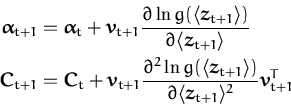
Appendix F. Using the differential of the
log-averages with respect to the prior mean vector at time t + 1, we
have the updates for the GP parameters
) and its derivatives to
Appendix F. Using the differential of the
log-averages with respect to the prior mean vector at time t + 1, we
have the updates for the GP parameters
![]() and
C:
and
C:
and
![]() zt + 1
zt + 1![]() is 2×1 a vector, implying vector and matrix
quantities in (175). The matrices
K0[t + 1] and
I[t + 1]2 are shown in Fig. 5.11.
is 2×1 a vector, implying vector and matrix
quantities in (175). The matrices
K0[t + 1] and
I[t + 1]2 are shown in Fig. 5.11.
|
Fig. 5.12 shows the results of the online algorithm applied on a sample wind field having 100 nodes on an equally spaced lattice. In subfigure (a) the predictions from the Numerical Weather Prediction (NWP) are shown as a reference to our online GP predictions, shown in sub-figures (b)-(d). The processing order of each node appears to be important for this case: depending on the order we have a solution agreeing with the NWP results as shown in sub-figures (b) and (d), on other occasions the online GP had a clearly suboptimal wind field structure, as shown in subfigure (d).
However, we know that the posterior distribution of the wind field given the scatterometer observations is multi-modal, with in general two dominating and well separated modes.
The variance in the predictive wind fields resulting from different presentation orders is a problem for the online solutions: we clearly do not know in advance the preferred presentation order, and this means that there is a need to empirically assess the quality of each resulting wind field, this will be presented in the next section.
An exact computation of the posterior process, as it has been discussed previously, would lead to a multi-modal distribution of wind fields at each data-point. This would correspond to a mixture of GPs as a posterior rather than to a single GP that is used in our approximation. If the individual components of the mixture are well separated, we may expect that our online algorithm will track modes with significant underlying probability mass to give a relevant prediction. However, the mode that will be tracked depends on the actual sequence of data-points that are visited by the algorithm. To investigate the variation of our wind field prediction with the data sequence, we have generated several random sequences and compared the outcomes based on a simple approximation for the relative mass of the multivariate Gaussian component.
To compare two posterior approximations obtained from different
presentations of the same data, we assume that the marginal
distribution
(![]() ,
,![]() ) can be written as a sum of
Gaussians that are well separated. At the online solutions
) can be written as a sum of
Gaussians that are well separated. At the online solutions
![]() we are at a local maximum of the pdf, meaning that the sum from the mixture of Gaussians is reduced to a single term.
This means that
we are at a local maximum of the pdf, meaning that the sum from the mixture of Gaussians is reduced to a single term.
This means that
with
q(![]() ) from eq. (170),
) from eq. (170),
![]() the weight of the component of the mixture
to which our online algorithm had converged, and we assume the local
curvature is also well approximated by
the weight of the component of the mixture
to which our online algorithm had converged, and we assume the local
curvature is also well approximated by
![]() .
.
Having two different online solutions
(![]() ,
,![]() )
and
(
)
and
(![]() ,
,![]() ), we find from eq (176) that
the proportion of the two weights is given by
), we find from eq (176) that
the proportion of the two weights is given by
as illustrated in Fig. 5.13. This helps us to estimate the ``relative weight'' of the wind field solutions:
helping us to assess the quality of the approximation we
obtained. Results, using multiple runs on a wind field data confirm
this expectation, the correct solution (Fig. 5.14.b)
has large value and high frequency if doing multiple runs. For the
wind field example shown in Fig. 5.12 100 random
permutations of the presentation were made. The resulting good
solutions, shown in subfigure (b) and (c) always had the logarithm of
the relative weight larger than 90 whilst the bad solutions had the
same quantity at
![]() 70.
70.
The sparsity for the vectorial GP is also based on the same
minimisation of the KL-distance, as for the scalar GPs. The only
difference from Chapter 3 is that here we have a
vectorial process. Using the transformed notations from
eq. (173), the vectorial GP means that the removal and
addition operations can only be performed in pairs. The
![]() set, for
the transformed GP has always an even number of basis vectors: for
each spatial location
xi the
set, for
the transformed GP has always an even number of basis vectors: for
each spatial location
xi the
![]() set includes
xiu and
xiv. If removing
xi, we have to remove both components
from the
set includes
xiu and
xiv. If removing
xi, we have to remove both components
from the
![]() set. The pruning is very similar to the one-dimensional
case. The difference is that the elements of the update are 2×2 matrices (
c* and
q*), p×2 vectors (
C* and
Q*), and the 2×1 vector
set. The pruning is very similar to the one-dimensional
case. The difference is that the elements of the update are 2×2 matrices (
c* and
q*), p×2 vectors (
C* and
Q*), and the 2×1 vector
![]() *, the decomposition is
the same as showed in Fig. 3.3. Using this decomposition
the KL-optimal updates are
*, the decomposition is
the same as showed in Fig. 3.3. Using this decomposition
the KL-optimal updates are
where
Q-1 is the inverse Gram matrix and
(![]() ,C) are
the GP parameters.
,C) are
the GP parameters.
The quality of the removal of a location xi (or the two virtual basis vectors xiu and xiv) is measured by the approximated KL-distance from Chapter 3, leading to the score
where the parameters are obtained from the 2N×2N matrix using the same decomposition shown in Fig 3.3.
|
The results of the pruning are promising: Fig. 5.14 shows the resulting wind field if 85 of the spatial knots are removed from the presentation eq. (173). On the right-hand side the evolution of the KL-divergence and the sum-squared errors in the means between the vector GP and a trimmed GP using eq. (179) are shown as a function of the number of deleted points. Whilst the approximation of the posterior variance decays quickly, the predictive mean is stable when deleting nodes.
The sparse solution from Fig. 5.14 is the result of combining the non-sparse online algorithm with the KL-optimal removal, the two algorithms being performed one after the another. This means that we still have to store the full vector GP and the costly matrix inversion is still needed, the difference from other methods is that the inversion is sequential.
Applying the sparse online algorithm without the EP re-learning steps lead to significant loss in the performance of the online algorithm, this is due to the more complex multimodal ``likelihoods'' provided by the MDNs that give rise to local symmetries in the parameter space. We compensated for this loss by using additional prior knowledge. The prior knowledge was the wind vector at each spatial location from a NWP model and we included this in the prior mean function. This leads to better performance since we are initially closer to the solution than using simply a zero-mean prior process. The performance of the resulting algorithm is comparable to the combination of the full online learning with the removal and the result is shown in Fig. 5.14.b.
For the wind-field example the EP algorithm from Chapter 4 has not been developed yet. Future work will involve testing the sparse EP algorithm applied to the wind-field problem. As seen for the classification case, the second and third iteration through the data improved the performance. By performing the multiple iterations for the spatial locations we expect to have a better approximation for the posterior GP for this case also. Some improvement is also to be expected when estimating the relative weight of a solution from eq. (178), especially since here an accurate estimation of the posterior covariance is essential.
To conclude, we showed that the wind-field approximation using sparse GPs is a promising research direction. We showed that a reduction of 70% of the basis points lead to a minor change in the actual GP, measured using the KL-distance. The implementation and testing of the sparse EP algorithm for this special problem is also an interesting question.
We estimated the wind-fields by first processing the raw scatterometer
data using the local inverse models into a mixture of Gaussians as
shown in Fig 5.10. The GP learning algorithm used the
product of these local mixtures. Further investigations are aimed at
implementing the GPs based on likelihoods directly from the
scatterometer observations. Since the dependence of the wind-field on
the scatterometer observation is given by a complex forward model, we
need to perform approximations to compute
g(![]() z
z![]() ) and to
benchmarks the results with previous ones.
) and to
benchmarks the results with previous ones.
A modification of the model in a different direction is suggested by the fact that the mixtures tend to have two dominant modes, this resulting from the physics of the system. The same bimodality has also been found in empirical studies [48]. It would be interesting to extend the sparse GP approach to mixtures of GPs in order to incorporate this simple multi-modality of the posterior process in a principled way.
We presented results for various problems solved using the sparse GP
framework with the aim of showing the applicability of the algorithm
to a large class of likelihoods. Sparseness for the quadratic
regression case showed performance comparable with the full GP
regression, tested with artificial and real-world datasets. The
additional EP iterations were beneficial only if the
![]() set size was
very low, but generally did not improved the test errors. This was
not the case for the classification problems, where we showed both the
applicability of the sparse GP learning and the improved performance
with multiple sweeps through the data. The performance of the
algorithm with the classification problem was also tested on the
relatively large USPS dataset having 7000 training data. Despite of
the fact that only a fraction of the data was retained, we had good
performance. An interesting research direction is to extend sparse GP
framework to the robust regression, i.e. non-Gaussian noise
distributions like Laplace noise. However, we believe that this would
be beneficial only if a method of hyper-parameter selection could be
proposed.
set size was
very low, but generally did not improved the test errors. This was
not the case for the classification problems, where we showed both the
applicability of the sparse GP learning and the improved performance
with multiple sweeps through the data. The performance of the
algorithm with the classification problem was also tested on the
relatively large USPS dataset having 7000 training data. Despite of
the fact that only a fraction of the data was retained, we had good
performance. An interesting research direction is to extend sparse GP
framework to the robust regression, i.e. non-Gaussian noise
distributions like Laplace noise. However, we believe that this would
be beneficial only if a method of hyper-parameter selection could be
proposed.
The application of the GPs to density estimation at the present time is very restrictive: we considered one-dimensional data and special kernels. For this case the EP steps proved to be very important, several iterations were needed to reach a reasonable solution. However the solution is attractive: we showed the possibility to infer multi-modal distributions without specifying the number of peaks in the distribution.
A real-world application is the sparse GP inference of wind-fields
from scatterometer observations. Previous studies [13]
shown that this problem in not unimodal, our sparse GP tracks a mode
of the posterior distribution. This being a work in progress, we
expect more positive results from the implementation and testing of
the EP algorithms for the wind fields. Discussion about more general
future research topics like model selection can be found in the next
chapter.

![\includegraphics[]{sinc_POL_5_0.02.eps}](img612.png)
![\includegraphics[]{sinc_RBF_10_1_0.02.eps}](img613.png)

 +
+ ![\includegraphics[]{bo_RBF_2_3_0.01_481_norm.eps}](img624.png)
![\includegraphics[]{bo_RBF_2500_1_5e-05_481.eps}](img625.png)

![\includegraphics[]{crab_RBF_2_4_0.01_80.eps}](img653.png)
![\includegraphics[]{crab_RBF_2_4_0.01_80_frag.eps}](img654.png)
![\includegraphics[]{son_RBF_0.25_1_0.0001_104.eps}](img656.png)
![\includegraphics[]{son_RBF_0.25_1_0.0001_104_frag.eps}](img657.png)
![\includegraphics[]{usps4_RBF_0.5_2_10.eps}](img660.png)
![\includegraphics[]{usps_all_RBF_0.5_2.eps}](img661.png)
![\includegraphics[]{usps_reject_RBF_0.5_2_150.eps}](img662.png)
![\includegraphics[]{usps_reject_RBF_0.5_2_350.eps}](img663.png)

 with Z =
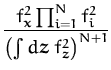
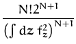


![$\displaystyle {\frac{\int d{\boldsymbol { x } }\; E_{\lambda_m}\left[ f_{\bolds...
...2 \prod_{i=1}^N f_i^2 \right]}{E_{\lambda_m}\left[\prod_{i=1}^N f_i^2 \right]}}$](img709.png) .
.![$\displaystyle {\frac{E_\lambda\left[ f_{\boldsymbol { x } }^2 \prod_{i=1}^N f_i^2 \right]}{E_\lambda\left[\prod_{i=1}^N f_i^2 \right]}}$](img711.png) .
.![\includegraphics[]{sinc_kernel.eps}](img723.png)
 exp
exp
![\includegraphics[]{FSIN_6_500_20sweeps_GOOD.eps}](img756.png)
![\includegraphics[]{sinc_dens_plateau.eps}](img757.png)
 and W0(x,y) =
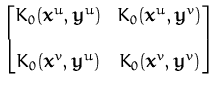
![\includegraphics[]{schematic.eps}](img777.png)

 with vt + 1 = CtK0[t + 1] + I[t + 1]2
![\includegraphics[]{NWP_all.eps}](img783.png)
![\includegraphics[]{Online_most_frequent.eps}](img784.png)
![\includegraphics[]{symm_sol.eps}](img785.png)
![\includegraphics[]{bad_sol_49_84.eps}](img786.png)
![\includegraphics[]{rel_weight.eps}](img787.png)
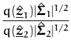

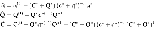
![\includegraphics[]{85_rem_13.eps}](img803.png)
![\includegraphics[]{KL_sq_13.eps}](img804.png)