In this section we obtain the coefficients for the online update of
the vectorial GP from Section 5.4. For this we need a
single likelihood term, indexed t, and the vector GP marginal at
time t - 1, denoted
qt - 1(z) where z is the two-dimensional wind
vector. The single ``likelihood'' term has a mixture of 4 Gaussians
(following the description from [22])
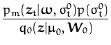
pm(zt|![]() ,
,![]() ) =
) = ![]()
![]()
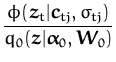
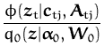
![]() (zt|ctj,
(zt|ctj,![]() ) in the numerator and the
GP marginal at
xt, a two-dimensional Gaussian denoted
q0(z|
) in the numerator and the
GP marginal at
xt, a two-dimensional Gaussian denoted
q0(z|![]() 0,W0) in the denominator:
0,W0) in the denominator:
with the mixture coefficients
![]()
![]() = 1 and
= 1 and
![]() (zt|ctj,
(zt|ctj,![]() ) is one component of the
Gaussian mixture: a spherical Gaussian centered at
ctj and
with spherical variance
) is one component of the
Gaussian mixture: a spherical Gaussian centered at
ctj and
with spherical variance
![]() I2 = Atj. We will
use zero prior mean functions, thus we do not write
I2 = Atj. We will
use zero prior mean functions, thus we do not write
![]() 0 in what
follows.
0 in what
follows.
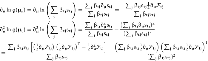
We need to compute the average of the likelihood in
eq. (220) with respect to the Gaussian
qt - 1(z|![]() t,Wt) where
(
t,Wt) where
(![]() t,Wt) are
the mean and variance of the GP marginal at
xt. Using these
notations we write the required average as:
t,Wt) are
the mean and variance of the GP marginal at
xt. Using these
notations we write the required average as:
where the dependence on the mean of the GP marginal
![]() t is
explicitly written. We decompose eq. (221) into the
sum:
t is
explicitly written. We decompose eq. (221) into the
sum:
and in the following we compute
stj(![]() t). We have the
same integral for each
stj(
t). We have the
same integral for each
stj(![]() t), we remove the indices
and compute a generic
t), we remove the indices
and compute a generic
All distributions involved are Gaussian, the resulting distribution thus will also be a Gaussian one with the general form:
| s = K exp(- |
with the quadratic term
or equivalently (using the matrix inversions from eq. (181)):
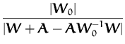
and the multiplying constant
The first and second order differentials of ![]() :
:
We can substitute back each
stj(![]() t) = Ktjexp(-
t) = Ktjexp(- ![]() tj/2) and differentiate
log g(
tj/2) and differentiate
log g(![]() t) with respect
to
t) with respect
to
![]() t to get the quantities required for the updates of the
vector GP in eq. (175):
t to get the quantities required for the updates of the
vector GP in eq. (175):
where
![]() stj is the responsbility of the j-th component
of the mixture for generating data
xt.
stj is the responsbility of the j-th component
of the mixture for generating data
xt.
 =
= 
 qt - 1(z|
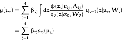
 qt - 1(z|
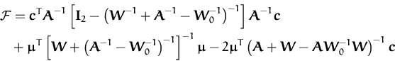
 .
.![\begin{displaymath}\begin{split}\frac{1}{2} \partial_{\boldsymbol { \mu } }{\cal...
...{\boldsymbol { W } }_0^{-1}\right)^{-1}\right]^{-1} \end{split}\end{displaymath}](img933.png) .
.