The sparse online GPs of the previous chapter (presented in Section 3.6) can process arbitrarily large datasets. This is possible by avoiding the increase of the GP parameter set using KL-projections to a constrained family of GPs. The drawback of the algorithm stems from its online nature: each example can be processed only once. Indeed, when using the same example in a second iteration there are artifacts caused by treating the already seen data point as independent from the model. This single iteration also means that the solution is dependent on the order of the presentation of the inputs, an unwanted result. If the size of the data is large, then it can be argued that the resulting GP becomes independent of the ordering, but the single processing is disadvantageous if we want to improve the GP when we have smaller datasets and enough computational power for multiple processing.
Recently, an extension to the online learning was proposed by [46], named the expectation-propagation (EP) algorithm. This algorithm improves the result of the Bayes online learning by making possible additional processing of the examples. The algorithm stores the contribution of each example to the approximated posterior. At each online learning step, before processing a data likelihood, the contribution of that specific example is first ``subtracted'' from the approximated posterior. The result is a fixed-point iterative algorithm that repeatedly processes each single data likelihood and converges to a solution that is independent of the order the data is processed. The EP algorithm stops when there are no changes in the individual contributing terms for a full cycle through the data. It has been shown in [46] that the fixed point of the algorithm coincides with the fixed point of the TAP approximation, a statistical physics method that was applied to approximate the posteriors [53], more details in Section 4.2.
The EP algorithm was applied to GPs and it showed improvements over the single-sweep online learning [46]. The EP algorithm in its original form also suffers from the bad scaling of GPs, being of restricted use. In this chapter we combine the EP and the sparse online algorithm for the GPs.
The EP algorithm is discussed in Section 4.1 and then applied to GPs in Section 4.2. The EP algorithm induces an alternative parametrisation to the posterior GP: it is written as the prior and a product of conjugates of the posterior family, the contribution of the individual examples. The connection between the EP-parametrisation and the one based on the parametrisation lemma is presented in Section 4.3. The equivalence of the parametrisations provides the ground for extending the sparse projection method to the EP algorithm (Section 4.4). The algorithm is sketched in Section 4.6 and the chapter finishes with conclusions and discussions.
Expectation-propagation (EP) [46] is based on the
Bayesian online learning presented in Chapter 2 (also
in [25]). Since EP exploits and extends the iterations
in the online learning, we first sketch online learning and then
present the EP algorithm. Let us denote with
![]()
![]()
![]() m the set of model parameters. We want to infer their
distribution
q(
m the set of model parameters. We want to infer their
distribution
q(![]() ). The prior over the parameters is
q0(
). The prior over the parameters is
q0(![]() ) and, as previously, we assume a factorising likelihood:
) and, as previously, we assume a factorising likelihood:
where
{(x1,y1),...,(xN,yN)} is the data set and
![]() (yi,xi|
(yi,xi|![]() ) is the likelihood function. To
simplify the notation, in the following the inputs
(xk,yk) will be
suppressed from the likelihood function, being encoded in its index.
) is the likelihood function. To
simplify the notation, in the following the inputs
(xk,yk) will be
suppressed from the likelihood function, being encoded in its index.
We denote by
q(n)(![]() ) the Bayesian posterior obtained from
including all data points up to, and including index n:
) the Bayesian posterior obtained from
including all data points up to, and including index n:
and observe that we have a recursive relation:
In Chapter 2 different approximation techniques to the
intractable posterior have been presented
(section 2.2.2) with the focus on online learning:
eq. (52) [55]. In Bayesian online
learning the approximation to the true posterior
qpost(N)(![]() ) including all examples is obtained by a
succession of approximating steps to compute
) including all examples is obtained by a
succession of approximating steps to compute
![]() (
(![]() ),
an approximation to
qpost(n)(
),
an approximation to
qpost(n)(![]() ).
).
This is an iterative procedure where we use
![]() (
(![]() ), the result from the previous online
approximation. The posterior is found by applying
eq. (99) with
), the result from the previous online
approximation. The posterior is found by applying
eq. (99) with
![]() (
(![]() ) instead of
q(n - 1)(
) instead of
q(n - 1)(![]() ). Since
q(n)post is also intractable, a
second approximation step is used to obtain
). Since
q(n)post is also intractable, a
second approximation step is used to obtain
![]() . This is
formally written as
. This is
formally written as
where the arrow specifies a projection of the intractable posterior to
a tractable family of distributions. Performing the iterations for
all data gives
![]() which depends on the order of presentation.
Unless new data arrives it is impossible to improve on the
online result.
which depends on the order of presentation.
Unless new data arrives it is impossible to improve on the
online result.
The goal of expectation propagation is to apply further
iterations of the updates for the posterior distribution, thus
producing a better approximation than the result from online algorithm
alone. To achieve this, we ``unfold''
![]() , the end-result
of the online iterations, as
, the end-result
of the online iterations, as
The observation made by [46] is that each factor in
the product corresponds to an approximation of the corresponding
likelihood term, since that has been the basis of the update
for
![]() from eq. (100). In the
following
from eq. (100). In the
following
![]() (
(![]() ) =
) = ![]() (
(![]() )/
)/![]() (
(![]() ) will be used and we will call this ratio as
approximating likelihood.
) will be used and we will call this ratio as
approximating likelihood.
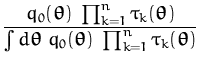
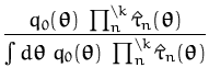
Using these notations, the Bayesian update is rewritten as a problem
of estimating the individual factors
![]() (
(![]() ) which give
the approximate posterior distribution:
) which give
the approximate posterior distribution:
The above relation is usable only if the prior distribution and the
approximated posterior belong to the family of the exponential
distributions [3]. Then, since it is the ratio of two
exponentials, the approximating likelihood is also in the exponential
family:
![]() (
(![]() ) is conjugate to the prior. The
approximating likelihoods used with the prior distribution lead to a
tractable posterior, without the need for any approximation. Further
we see the possible benefits of using the approximating likelihoods:
the approximations to
) is conjugate to the prior. The
approximating likelihoods used with the prior distribution lead to a
tractable posterior, without the need for any approximation. Further
we see the possible benefits of using the approximating likelihoods:
the approximations to
![]() (
(![]() ) are made locally, weighted
by
) are made locally, weighted
by
![]() (
(![]() ).
).
To improve on each term
![]() (
(![]() ) using online
learning, we first have to find the distribution
) using online
learning, we first have to find the distribution
![]() =
= ![]() (
(![]() ) independent of the
likelihood
) independent of the
likelihood
![]() (
(![]() ). This is done by removing
). This is done by removing
![]() (
(![]() ) from the posterior eq. (102).
This implies that we have to keep the approximated likelihoods for all
data. The online learning used here was presented in
Chapter 2. It minimises a
KL-distance [14] by matching the moments of the true
and the approximated posterior (see Section 2.2.2).
) from the posterior eq. (102).
This implies that we have to keep the approximated likelihoods for all
data. The online learning used here was presented in
Chapter 2. It minimises a
KL-distance [14] by matching the moments of the true
and the approximated posterior (see Section 2.2.2).
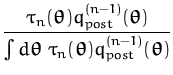
If an input
![]() (
(![]() ) has already been seen, we need to remove
its contribution
) has already been seen, we need to remove
its contribution
![]() (
(![]() ) from the current parameter
estimate before using the online step from Section 2.4.
This is done by ``subtracting'' it from the posterior and the online
learning rule is performed with the adjusted prior:
) from the current parameter
estimate before using the online step from Section 2.4.
This is done by ``subtracting'' it from the posterior and the online
learning rule is performed with the adjusted prior:
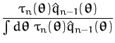
where the second term on the right does not depend on
![]() , the
parameter being integrated out. Using the modified prior
, the
parameter being integrated out. Using the modified prior
![]() and the likelihood-term
and the likelihood-term
![]() (
(![]() ),
the posterior
),
the posterior
![]() (
(![]() ) is:
) is:
Since
![]() (
(![]() ) appears both in the numerator and the
denominator, its normalising constants are irrelevant. This means
that in the numerical implementation of the algorithm it will be
enough to store the terms of the exponentials of
) appears both in the numerator and the
denominator, its normalising constants are irrelevant. This means
that in the numerical implementation of the algorithm it will be
enough to store the terms of the exponentials of
![]() . On the
other hand, an exact computation of each normalising constant would be
required if we want to approximate the evidence of the model,
considered by [46]. In this thesis the model selection
issue is not addressed, however, it is a very important area of future
research. The new
. On the
other hand, an exact computation of each normalising constant would be
required if we want to approximate the evidence of the model,
considered by [46]. In this thesis the model selection
issue is not addressed, however, it is a very important area of future
research. The new
![]() is computed as
is computed as
In the EP iterations we choose - randomly or by using different
heuristics - an index k and apply online learning for that example.
The cycle terminates if there are no changes in the approximated
likelihoods
![]() (
(![]() ). We do not have a guaranteed global
convergence but the system usually finds a fixed point and this
minimum point is independent of the order of inclusion of the
individual likelihoods.
). We do not have a guaranteed global
convergence but the system usually finds a fixed point and this
minimum point is independent of the order of inclusion of the
individual likelihoods.
![\includegraphics[]{ep_expl.eps}](img462.png)
|
The visualisation of the EP algorithm with the approximate likelihoods
![]() (
(![]() ) is shown in Fig. 4.1. Whilst in the
usual online learning at the end of the N-th iterations
) is shown in Fig. 4.1. Whilst in the
usual online learning at the end of the N-th iterations
![]() (
(![]() ) is the approximated posterior, in this case the
online steps are used to improve on the approximation of the
individual ``segments''
) is the approximated posterior, in this case the
online steps are used to improve on the approximation of the
individual ``segments''
![]() that build up
that build up
![]() (
(![]() ). The similarity of Fig. 4.1 with online
learning as presented in Fig. 2.2 illustrates that the EP
algorithm is built on the online method. The underlying dynamics is
different in the two cases: for online learning we have only the
``path'' toward the final approximation. In contrast, for the EP
algorithm the emphasis is on building up the chain that links the
prior with the posterior. If we take logarithms in
eq. (102), then
). The similarity of Fig. 4.1 with online
learning as presented in Fig. 2.2 illustrates that the EP
algorithm is built on the online method. The underlying dynamics is
different in the two cases: for online learning we have only the
``path'' toward the final approximation. In contrast, for the EP
algorithm the emphasis is on building up the chain that links the
prior with the posterior. If we take logarithms in
eq. (102), then
![]() is the difference between
two log-probabilities. Further, if we consider
is the difference between
two log-probabilities. Further, if we consider
![]() and
and
![]() as points in the space of distributions, then
as points in the space of distributions, then
![]() is a one-dimensional line connecting the two distributions, as shown
in Fig. 4.1. A first online sweep is used to initialise the
individual terms
is a one-dimensional line connecting the two distributions, as shown
in Fig. 4.1. A first online sweep is used to initialise the
individual terms
![]() . Alternatively the terms can be
initialised with a constant value 1, having
p0 =
. Alternatively the terms can be
initialised with a constant value 1, having
p0 = ![]() in the
beginning.
in the
beginning.
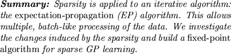
To sum up, the EP extension of the online learning algorithm from Chapter 2 implies:
The benefit of the EP algorithm is that it allows data processing beyond online learning, the extra cost, apart from the increased computational time, is the additional storage of the projected likelihood terms. The EP algorithm will be applied to GPs in the next section.
In the following the feature-space notation and the GP parametrisation from the parametrisation lemma 2.3.1 is used. Similarly to the intuition behind deducing the KL-divergences, the feature space formalism provides us with a more intuitive picture of the algorithm. The EP algorithm applied to GP classification was presented in [46, Chapter 5]. In this chapter we will leave the likelihood unspecified, the EP procedure being identical for other likelihoods also.
We assume that we are given the kernel
K0(x,x![]() ) and we consider
the feature space
) and we consider
the feature space
![]()
![]() and the scalar product generated by the kernel:
if
and the scalar product generated by the kernel:
if
![]() is the projection of the
x into the unknown
is the projection of the
x into the unknown ![]() , then we have
K0(x,x
, then we have
K0(x,x![]() ) =
) = ![]()
![]() [95,93]. Using
the feature space, the GP is equivalent to normal distribution for the
parameter vector
f in
[95,93]. Using
the feature space, the GP is equivalent to normal distribution for the
parameter vector
f in
![]()
![]() :
:
![]() , as shown
in Chapter. 2, eq. (48).
, as shown
in Chapter. 2, eq. (48).
![]() is a normal distribution with mean and covariance
given by:
is a normal distribution with mean and covariance
given by:
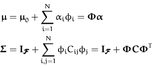
with
![]() = [
= [![]() ,...,
,...,![]() ]T,
C = {Cij}i, j = 1, N the parameters of the GP and
]T,
C = {Cij}i, j = 1, N the parameters of the GP and
![]() = [
= [![]() ,...,
,...,![]() ]T is the concatenation of all feature
vectors from the
]T is the concatenation of all feature
vectors from the
![]() set and
set and
![]() is the identity matrix in the
feature space. In the following we assume
is the identity matrix in the
feature space. In the following we assume
![]() = 0. At this point we also assume that the learning rules
do not include sparsity and the set of basis vectors coincides with
the input data, the sparse case being discussed later in
Section 4.4.
= 0. At this point we also assume that the learning rules
do not include sparsity and the set of basis vectors coincides with
the input data, the sparse case being discussed later in
Section 4.4.
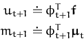
We use the ``time'' index t, and assume that
![]() (f)
is a likelihood chosen from the data set. The online updates,
assuming that
(f)
is a likelihood chosen from the data set. The online updates,
assuming that
![]() (f) was not previously processed, are
(eq. 54):
(f) was not previously processed, are
(eq. 54):
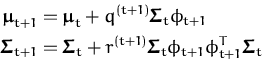
with
![]()
![]()
![]() and the scalars q(t + 1)
and r(t + 1) given in eq. (53). We have
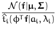
to find the approximate likelihood
and the scalars q(t + 1)
and r(t + 1) given in eq. (53). We have
to find the approximate likelihood
![]() (f), the ratio
of the approximated posterior GPs at time t + 1 and t respectively.
From the definition of
(f), the ratio
of the approximated posterior GPs at time t + 1 and t respectively.
From the definition of
![]() in eq. (102) we
have:
in eq. (102) we
have:
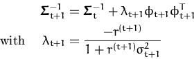
To simplify the expression for
![]() , we
first express the update rule for the inverse covariances in the
feature space using the matrix inversion lemma (eq. (181)
and [43]):
, we
first express the update rule for the inverse covariances in the
feature space using the matrix inversion lemma (eq. (181)
and [43]):
where
![]() =
= ![]()
![]()
![]() = k* + kt + 1TCkt + 1 is the
predictive variance of the GP at time t and at location
xt + 1.
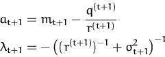
We define
= k* + kt + 1TCkt + 1 is the
predictive variance of the GP at time t and at location
xt + 1.
We define
the projection of the random variable
f and the mean where the
projection vector is
![]() . The exponential term
in (108) is rewritten as
. The exponential term
in (108) is rewritten as
and the ratio of the determinants becomes
leading to a scalar quadratic expression for the approximated likelihood
The parameters at + 1 and
![]() depend on the likelihood and the prior GP:
depend on the likelihood and the prior GP:
For a single likelihood this approximation is a one-dimensional
Gaussian in the random variable ut + 1. Since model selection is
not treated here, we do not have to store the normalising constants
for the posterior either. We have to keep only the parameters of the
distribution of ut + 1, that is the pair
(![]() , at + 1).
The cost is small, requiring 2N scalars. Using again
Fig. 4.1 we identify the segment from any
, at + 1).
The cost is small, requiring 2N scalars. Using again
Fig. 4.1 we identify the segment from any ![]() to
to
![]() as pointing to the direction of
as pointing to the direction of
![]() and
parametrised using
(
and
parametrised using
(![]() , at + 1).
, at + 1).
The prior GP and the approximated likelihood identify the approximated
posterior GP; this involves another data-dependent parametrisation.
In the following we assume that both the GP parameters
(![]() ,C)
and the scalars
(ai,
,C)
and the scalars
(ai,![]() ) are updated, the relation between
the two parametrisations is discussed in
Section 4.3.
) are updated, the relation between
the two parametrisations is discussed in
Section 4.3.
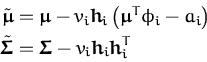
To perform the online update eqs. (107), first we
need to subtract the contribution of the current likelihood from the
model. We assume that an example
(xi,yi) has been picked for
processing and the approximated likelihood has the parameters
(ai,![]() ). We compute the new GP with
(
). We compute the new GP with
(![]() ,
,![]() ) given by the parametrisation
lemma 2.3.1:
) given by the parametrisation
lemma 2.3.1:
 |
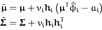
Matching the linear and quadratic terms in f leads to
giving us the parameters of the Gaussian with which we can perform the
online updates. The next step is to find the changed parameters
(![]() ,
,![]() ) of the new GP according to the
parametrisation lemma 2.3.1. By substituting the general
parametrisation from eq. (106) into
eq. (115) we find:
) of the new GP according to the
parametrisation lemma 2.3.1. By substituting the general
parametrisation from eq. (106) into
eq. (115) we find:
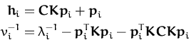
where
ki = [K0(x1,xi),..., K0(xN,xi)]T and
![]() = K0(xi,xi) + kiTCki is the variance of
the marginalisation of the GP at
xi.
= K0(xi,xi) + kiTCki is the variance of
the marginalisation of the GP at
xi.
The EP algorithm for the Gaussian processes can now be established.
We select the prior kernel and set
![]() = 0 and
C = 0.
Similarly, the additional parameters ai and
= 0 and
C = 0.
Similarly, the additional parameters ai and ![]() that
parametrise the likelihood approximations at the data points are also
set to zero. We mention that the zero value for
that
parametrise the likelihood approximations at the data points are also
set to zero. We mention that the zero value for ![]() simply
means vi = 0 in eqs. (115)
and (116).
simply
means vi = 0 in eqs. (115)
and (116).
After selecting an example
(xt + 1,yt + 1), the approximated
likelihood is subtracted from the GP, using eq (116).
Then we compute the scalar update coefficients q(t + 1) and
r(t + 1) using the ``corrected'' GP and the likelihood
t(xt + 1|f) applying the standard online learning
procedure, eq. (53). Simultaneously to the
online update for the GP parameters
(![]() ,C) from
eq. (57), we also update the coefficients of the
projected likelihoods
,C) from
eq. (57), we also update the coefficients of the
projected likelihoods
![]() (xt + 1) using
eqs. (114). The algorithm then processes a subsequent
example and stops if none of the parameters
(ai,
(xt + 1) using
eqs. (114). The algorithm then processes a subsequent
example and stops if none of the parameters
(ai,![]() ) are
changed.
) are
changed.
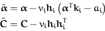
The EP algorithm encodes the approximated posterior in the one-dimensional normal distributions and we have to store the mean and the variance. In the statistical physics framework, mean field theory is an approximation technique that uses a simpler parametric form for the posterior distributions to obtain a tractable approximation. Recently mean field methods have been gaining popularity in the machine learning community; the techniques developed originally for statistical physics are applied to machine learning problems in [56]. The ADATAP approach [53] aims at finding the approximate posteriors for models using factorising likelihoods and prior distributions with quadratic terms, as is eq. (98) using Gaussian for p0(f). The random variables ui are termed cavity fields and a batch approximation for its distribution is provided using advanced statistical physics methods. The ADATAP method is not discussed here, we only mention that the fixed-point solution of the EP algorithm is the same as this approximation.
The EP learning, as presented in this section, applies to GPs that are
fully parametrised, i.e.. they include all data points in their
representation. To apply the EP for the sparse GP algorithm, we need
the updates for
(ai,![]() ) if an element from the
) if an element from the
![]() set is
removed. Before deriving the sparse EP algorithm, the relation
between the two representations for the same GP is established. The
sparse extension will follow from the relations between these two
parametrisations. The sparse extension of the EP algorithm will
follow from this equivalence, presented in Section 4.4
set is
removed. Before deriving the sparse EP algorithm, the relation
between the two representations for the same GP is established. The
sparse extension will follow from the relations between these two
parametrisations. The sparse extension of the EP algorithm will
follow from this equivalence, presented in Section 4.4
The posterior GP in the EP-framework is proportional to the prior GP
and the product of approximating likelihoods, providing an alternative
parametrisation to the GP. The EP representation in this case is via
N one-dimensional quadratic exponentials, the approximated
likelihood terms. The approximated likelihoods are defined in terms of
scalar random variables
ui = ![]() f which are projections of
f, the random variable in
f which are projections of
f, the random variable in
![]()
![]() . The resulting GP is written
as:
. The resulting GP is written
as:
where
![]() is a diagonal matrix having
is a diagonal matrix having ![]() on the
diagonals and
a is the vector of the means. The feature vectors
are grouped into
on the
diagonals and
a is the vector of the means. The feature vectors
are grouped into
![]() = [
= [![]() ,...,
,...,![]() ]T. We will call this
the ``EP-parametrisation''.
]T. We will call this
the ``EP-parametrisation''.
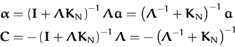
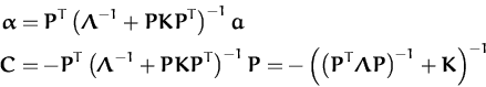
The second parametrisation of the same GP is given by the
parametrisation lemma and uses
(![]() ,C) as parameters of the
mean and the covariance as shown in eq. (106):
,C) as parameters of the
mean and the covariance as shown in eq. (106):
we term the ``natural parametrisation''. Since we have the same GP in
both cases, we can identify the coefficients of
f and
ffT in eqs. (117)
and (118):
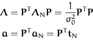
The matrix inversion lemma will transform the identities into a form
where we can identify the components. From the EP-parameters
(a,![]() ) we obtain the GP-ones
(
) we obtain the GP-ones
(![]() ,C) by
,C) by
where
KN is the kernel
matrix with respect to all data. Notice that the diagonal form of
![]() results from the factorising likelihood. The corresponding
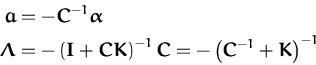
inverse relation is:
results from the factorising likelihood. The corresponding
inverse relation is:
Inspecting the above equations we see that the matrix
C is fully
specified by a diagonal matrix of the same size. This implies that we
can represent it by the diagonals of
![]() and use
eq. (119) whenever
C is needed. Apart from the
computational cost of this operation, in case of sparse updates this
simplification does not hold any more:
and use
eq. (119) whenever
C is needed. Apart from the
computational cost of this operation, in case of sparse updates this
simplification does not hold any more:
![]() is not diagonal
after removing some of the basis vectors, as will be shown in
the next section.
is not diagonal
after removing some of the basis vectors, as will be shown in
the next section.
Sparsity is defined using the ``natural parametrisation'' of
Chapter 2 with the parameters
(![]() ,C). The
sparse solution is obtained by eliminating some data points from the
representation while retaining as much information about the
data itself as possible. Using again the equivalence of GPs with
Gaussians in the feature space, we want the mean and covariance from
eq. (117) to be expressed, instead of the full data
vector
,C). The
sparse solution is obtained by eliminating some data points from the
representation while retaining as much information about the
data itself as possible. Using again the equivalence of GPs with
Gaussians in the feature space, we want the mean and covariance from
eq. (117) to be expressed, instead of the full data
vector
![]() = [
= [![]() ,...,
,...,![]() ]T, by using only a subset of it.
We follow the deduction of sparsity from Chapter 3: the
last element is removed from the
]T, by using only a subset of it.
We follow the deduction of sparsity from Chapter 3: the
last element is removed from the
![]() set, leaving
set, leaving
![]() =
= ![]()
![]() {
{![]() }. The derivation for the case of eliminating
more then a single element is very similar.
}. The derivation for the case of eliminating
more then a single element is very similar.
We assume that we have the EP-parameters
(a,![]() ) with respect
to the full input data
) with respect
to the full input data
![]() and we want to obtain the KL-optimal
parameters
(
and we want to obtain the KL-optimal
parameters
(![]() ,
,![]() ) using the restricted set
) using the restricted set
![]() of input features. We want to represent the resulting
GP using the EP-representation:
of input features. We want to represent the resulting
GP using the EP-representation:
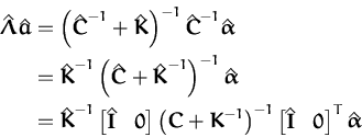
We start with deducing
![]() . For this we use the relation
between the EP-parameters and the natural parameters for the
covariance of the reduced system from eq. (122):
. For this we use the relation
between the EP-parameters and the natural parameters for the
covariance of the reduced system from eq. (122):
where we used the matrix inversion lemma eq. (181). We can now use the KL-optimal reduction of the matrix C from eq. (79)
 |
to replace
(![]() +
+ ![]() )-1. The matrix
[
)-1. The matrix
[![]() 0] is the concatenation of the identity matrix of
size N - 1 with a column of N - 1 zeroes.
The replacement leads to
0] is the concatenation of the identity matrix of
size N - 1 with a column of N - 1 zeroes.
The replacement leads to
The product
K [![]() 0]
0] ![]() = PN is an
orthogonal projection in the feature space
= PN is an
orthogonal projection in the feature space
![]()
![]() . The projection
eliminates the last component by orthogonally projecting it to the
span of the first N - 1 examples.
. The projection
eliminates the last component by orthogonally projecting it to the
span of the first N - 1 examples.
Next we consider the linear term in the EP-parametrisation of the GP
from eq. (117) with respect to
![]() f:
f:
![]() a. The sparse learning rules change it to
a. The sparse learning rules change it to
![]()
![]() and the new value is obtained from changes
in the natural parametrisation via eqs. (121)
and (122). We use, similarly to the case for the
quadratic term, the result from eq. (79) to relate the
reduced and the full EP-parameters of the GP:
and the new value is obtained from changes
in the natural parametrisation via eqs. (121)
and (122). We use, similarly to the case for the
quadratic term, the result from eq. (79) to relate the
reduced and the full EP-parameters of the GP:
where from line two to line three of the equation we replaced
(![]() +
+ ![]() ) with the corresponding expression from
eq. (79) using the old quantities. Similarly to the
case of the update of
) with the corresponding expression from
eq. (79) using the old quantities. Similarly to the
case of the update of
![]() we eliminate the pruned
we eliminate the pruned
![]() using eq. (77):
using eq. (77):
where
PN is again the projection matrix from
eq. (126). Substituting back the pruned coefficients
and using
![]() as the basis set, the projection matrix
PN is grouped with
as the basis set, the projection matrix
PN is grouped with
![]() and we have the
EP-parametrisation of the sparse GP from eq. (123) as
and we have the
EP-parametrisation of the sparse GP from eq. (123) as
This result says that by changing the feature vectors associated with
the likelihoods, we can keep the diagonal structure of the second
term. The index from the projection matrix
PN has been ignored
since it is straightforward that if successive projection steps are
used, the corresponding matrices multiply and we have, for each input
example, the approximation of the feature space image using only the
elements from
![]() :
:
![]() =
= ![]() pi =
pi = ![]()
![]() pij with
pij with ![]() being the i-th column of
P.
Similarly to the basic EP algorithm, the approximation
being the i-th column of
P.
Similarly to the basic EP algorithm, the approximation
![]() is used for the projection in obtaining the one-dimensional random
variable from eq. (110):
ui =
is used for the projection in obtaining the one-dimensional random
variable from eq. (110):
ui = ![]() f.
f.
The important result in eq. (129) is that the
sparse EP algorithm preserves the structure of the EP parametrisation,
the KL-optimal pruning changes ``only'' the directions of projecting
the approximating likelihoods, there are no modifications in
![]() or
or
![]() . This means that when iterating the pruning procedure
we have to store the successive projections of all data:
assuming a projection matrix, the ``update'' for it is
Pnew = PPold.
. This means that when iterating the pruning procedure
we have to store the successive projections of all data:
assuming a projection matrix, the ``update'' for it is
Pnew = PPold.
The multiplication of the orthogonal projections might suggest that
there is no need for memorising a large
P. Indeed, removing the
last element is done with
PN = K[![]() 0]
0]![]() .
If we remove one more element we use the matrix
PN - 1 =
.
If we remove one more element we use the matrix
PN - 1 = ![]() [
[![]() 0]
0]![]() with
with
![]() the Gram matrix containing N - 2 elements, then their multiplication
gives
P = K[
the Gram matrix containing N - 2 elements, then their multiplication
gives
P = K[![]() 0][
0][![]() 0]
0]![]() and if we know the N - 2 elements of
and if we know the N - 2 elements of
![]() then it might be
enough to store
then it might be
enough to store
![]() as in the previous chapter. This
is indeed the case if we do not add elements to
as in the previous chapter. This
is indeed the case if we do not add elements to
![]() set in
between the removals. Otherwise we must know the content of the
set in
between the removals. Otherwise we must know the content of the
![]() set when removing an element and keep track of the changes to this
particular subset.
set when removing an element and keep track of the changes to this
particular subset.
A first observation is that the storage of the projection matrix
P is needed, increasing the memory requirements from
![]() O(d2) to
O(d2) to
![]() (Nd + d2) where d is the size of the
(Nd + d2) where d is the size of the
![]() set.
set.
Secondly, we see that the KL-optimal pruning of a
![]() does not
mean that the approximated likelihood for that data is constant: the
direction of the projection is changed. In practise the successive
projections might mean the effective removal of a likelihood term, but
this is often not the case. The presence of the approximated
likelihood even for data which have been removed might justify the
good experimental results for the sparse online
learning [19].
does not
mean that the approximated likelihood for that data is constant: the
direction of the projection is changed. In practise the successive
projections might mean the effective removal of a likelihood term, but
this is often not the case. The presence of the approximated
likelihood even for data which have been removed might justify the
good experimental results for the sparse online
learning [19].
A third useful remark is the relation of the two GP-parametrisations in the sparse case. This is an obvious generalisation of the correspondence given in Section 4.3, eqns. (121) and (122) deduced for the non-sparse case:
The difference from the non-sparse case is that, due to the sparsity, the lemma-based representation alone cannot provide the EP-representation, the system is under-determined. In practise, eqns. (130) were used to check the correctness of the implemented code.6.
To summarise, the expectation-propagation for the sparse GP implies
the projection on a different direction of the random variable
f in the feature space. The change of the term ui from
eq. (110) implies that the result of the subtraction of
the approximated likelihood is different from
eq. (116). If an example
(xi,yi) is chosen,
then first we have to subtract the approximated likelihood from the
GP. The new parameters
(![]() ,
,![]() ) are:
) are:
and translated into the parameters
(![]() ,C), we have the
corrections to these parameters required before applying the online
updates as:
,C), we have the
corrections to these parameters required before applying the online
updates as:
where
K is the Gram matrix of the
![]() elements and
pi is
i-th column of the projection matrix
P.
elements and
pi is
i-th column of the projection matrix
P.
The sparse EP is a refinement of the sparse online algorithm, thus it is related to the kernel PCA methods [73] and the Nyström method proposed to speed up kernel machines [101]. In the following we compare the Nyström method applied for the regression case with the sparse EP algorithm.
The Nyström method uses the feature space
![]()
![]() and a subset from the
training set to construct an approximation to the eigenvalues of the
kernel function, presented in details in
Section 3.7. Using a subset of size m, there
will be only m nonzero approximated eigenfunctions. Assuming a data
set of size N, the N×N kernel matrix
KN is approximated
with the smaller-rank
and a subset from the
training set to construct an approximation to the eigenvalues of the
kernel function, presented in details in
Section 3.7. Using a subset of size m, there
will be only m nonzero approximated eigenfunctions. Assuming a data
set of size N, the N×N kernel matrix
KN is approximated
with the smaller-rank
where we used the projection matrix
P = kNmKm-1 from
the previous section and we assumed that the subset of size m for
the Nyström method is the
![]() set.
set.
In applications the inversion of the large KN is replaced with the inversion of the smaller matrix Km and the matrix inversion lemma from eq. (181) is exploited to reduce the cost of computations. For regression, where we know the analytical result, the Nyström method applied to computing the predictive mean at x is
where
kN = [K0(x1,x),..., K0(xN,x)]T,
![]() is the noise variance, and
tN is the vector of outputs.
is the noise variance, and
tN is the vector of outputs.
To compare it with the sparse EP algorithm, we assume a specific order
for the presentation of the data: the elements of the
![]() set are
presented first and there is no removal. This is equivalent with
applying the KL-projection to the full posterior process. For the
full process we have
set are
presented first and there is no removal. This is equivalent with
applying the KL-projection to the full posterior process. For the
full process we have
![]() N = IN/
N = IN/![]() and
aN = tN. We apply the KL-projection to the
and
aN = tN. We apply the KL-projection to the
![]() set, leading to the GP
with parameters in the EP representation:
set, leading to the GP
with parameters in the EP representation:
and similarly we compute the predictive mean for the sparse EP algorithm: where kBV = [K0(x1,x),..., K0(xm,x)]T. We interpret PkBV as the reconstruction of kN from eq. (134), and similarly PPTtN is an approximation to tN using the m available basis vectors. We write the expression corresponding to the predictive variance for the EP regression (using k* = K0(x,x)).
We see again that the predictive variance is also expressed using the
reconstructions of the inputs from the
![]() set. A similar
construction for the predictive variance in the Nyström method does not exist: we do not get positives variance at all input
points
x, the Nyström method is probabilistically inconsistent,
this is because it only considers the GP marginals at the data
locations.
Compared with the Nyström method, we see that the sparse EP
algorithm provides a less accurate posterior mean then the Nyström
method method, but it has the advantage of a fully probabilistic
treatment.
set. A similar
construction for the predictive variance in the Nyström method does not exist: we do not get positives variance at all input
points
x, the Nyström method is probabilistically inconsistent,
this is because it only considers the GP marginals at the data
locations.
Compared with the Nyström method, we see that the sparse EP
algorithm provides a less accurate posterior mean then the Nyström
method method, but it has the advantage of a fully probabilistic
treatment.
The algorithm proposed here has an increased complexity compared with
the sparse online algorithm and the same structure as the original
expectation-propagation [46]. Additional cost, compared
with the sparse online algorithm arises from the need to update the
P, the matrix of projections, that requires
![]() (Nd )
operations.
(Nd )
operations.
Similarly to the sparse online algorithm from
Section 3.6, we set the maximal
![]() set size in
advance to
M
set size in
advance to
M![]() . Whenever the size of the
. Whenever the size of the
![]() set gets larger then
M
set gets larger then
M![]() we delete the
we delete the
![]() with the smallest score. For algorithmic
stability we also use the tolerance value
with the smallest score. For algorithmic
stability we also use the tolerance value
![]() to prevent
the Gram matrix from being singular.
to prevent
the Gram matrix from being singular.
It starts with initialising the GP parameters
(![]() ,C) and
,C) and
![]() set with empty values, and also initialising the EP parameters
(ai,
set with empty values, and also initialising the EP parameters
(ai,![]() ) for all inputs with zero values. Since
) for all inputs with zero values. Since
![]() set
is empty, the projection matrix is also empty.
set
is empty, the projection matrix is also empty.
For a selected example (xi,yi) the algorithm iterates the following steps:
If
![]() <
< ![]() then perform the sparse updates.
then perform the sparse updates.
The algorithm is iterated until some convergence criterion is met or for a fixed number of sweeps through the whole data. In the experiments we employed the later choice. This seemed reasonable since a steady performance was reached in most cases after the second sweep through the data. A more detailed sketch of the algorithm is given in Appendix G, with related equations written explicitly.
This chapter developed an iterative approach to improve on the sparse
online solution such that the sparseness, i.e. the possibility of a
flexible treatment of the
![]() set size, is preserved.
set size, is preserved.
The improvement is based on the expectation-propagation algorithm for
the GPs, presented by [46]. Its extension to sparse GPs
increases the computational demand by requiring, beyond the parameters
(ai,![]() ), the storage of a projection matrix
P of size
N×d with d being the size of the
), the storage of a projection matrix
P of size
N×d with d being the size of the
![]() set.
set.
We believe that the EP algorithm for the sparse GPs fills in a gap in the applicability of GPs: if we have a small data set, then the EP algorithm proposed originally by [46] suffices. For the case of large datasets, we believe (as supported by experiments), that the sparse GP algorithm presented in Chapter 3 is the only available method if we want to use GPs. Additionally, there is a class of problems with data size that makes the EP algorithm inapplicable or inefficient, but for which the sparse online GP algorithm does not provide a sufficiently good solution. For these algorithms the EP extension of the sparse GPs can be used.
Further work needs to consider model selection for this class of algorithms. We have the ability to approximate the data likelihood, and this could provide us with an appropriate tuning of the hyper-parameters.
An interesting problem is the extensibility of the sparse framework to
non-Gaussian families. This is suggested by the observation that if
we use the
EP-representation, then minimising the KL-divergence translates into simple
projections of the examples to the set of basis vectors. Pruning is
then performed by writing the solution of the problem into the EP-form
of eq. (117), performing the removal of inputs in this
framework and transforming back into a more convenient representation.
 .
.
 .
.
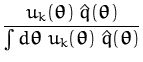 with uk(


![\begin{displaymath}\begin{split}\hat{t}_{t+1} &= \frac{{\ensuremath{{\mathcal{N}...
... { \mu } }_t-{\boldsymbol { f } }) \right] \right\} \end{split}\end{displaymath}](img479.png)

 .
. with
with 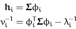
 with
with 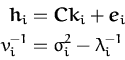
![\begin{displaymath}\begin{split}{\ensuremath{{\cal{GP}}}}_{post}({\boldsymbol { ...
...ymbol { f } }-{\boldsymbol { a } }) \right]\right\} \end{split}\end{displaymath}](img518.png)

 with
with 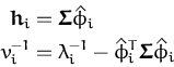
 with
with