Advances in computing capabilities have allowed increasingly complex learning procedures to be implemented in practical scenarios. In recent years there has been a growing interest in more powerful but demanding methods such as sampling techniques, non-parametric algorithms, boosting, or nearest-neighbour techniques. These methods are able to learn non-linear, i.e. more complex relationships in the data. Their limiting factor is the computational time: sampling techniques like Monte Carlo methods or particle filtering are costly since they require an extensive search in the parameter space when making predictions, leading to very long convergence times when applied for high-dimensional data sets.
Non-parametric methods, like various kernelised algorithms, provide the solutions as function of all training data, in this case the required memory scales with the size of the data set, implying both a prolonged computation and large storage requirement. The ongoing interest in their application is justified by the good performance of the non-parametric methods for real tasks, see e.g. [81], this performance usually being better then that of the semi-parametric neural networks [31]. However, the cost of an increased performance is the increased computational time, the basic (i.e. non-probabilistic) neural networks providing results in shorter time and without the need for an increased memory.
The complexity and the computational cost of a learning algorithm is also increased if one uses Bayesian probabilistic methods. Bayesian learning is a probabilistic parameter estimation method that uses Bayes theorem both to infer the distribution of the parameters from the data and to obtain the probabilistic prediction corresponding to an example.
In this thesis Bayesian learning is applied in the family of kernel
methods: we study inference using Gaussian processes (GPs). GPs
associate a random variable to each input location. For any finite set
of inputs the associated random variables are jointly Gaussian. The
GPs are thus random functions characterised by the mean and kernel functions. The kernel provides the covariance: each pair of
random variables at input locations
x and
x![]() has covariance
K0(x,x
has covariance
K0(x,x![]() ). Using GPs requires the manipulation of the
covariance matrix for the whole training set. The scaling of the
memory required for the GP is thus quadratic in the size of the
training data. The main problem when using GPs in practise is, as
with general kernel and non-parametric methods, the data dependent
scaling of the parameter space, scaling that is quadratic in the case
of Gaussian processes.
). Using GPs requires the manipulation of the
covariance matrix for the whole training set. The scaling of the
memory required for the GP is thus quadratic in the size of the
training data. The main problem when using GPs in practise is, as
with general kernel and non-parametric methods, the data dependent
scaling of the parameter space, scaling that is quadratic in the case
of Gaussian processes.
This thesis addresses the problem of efficient representation of a GP. The proposed representation uses only a fraction of the training data, and the size of this subset can be fixed before learning. Fixing the size of this subset extends the applicability of GPs to arbitrarily large datasets.
After an overview of Bayesian learning in the next section, we describe the application of this learning technique to GPs in Section 1.2. The problems faced when applying GPs to realistic data, and the solutions put forward in this thesis are also outlined.
The advantages of Bayesian methods over other methods stem from the probabilistic treatment of the problem. An immediate advantage is that we are able to estimate the uncertainty about a predicted output.
To apply Bayesian learning we assume a probabilistic framework for the
data: we consider the data likelihood. Let
xi ![]()
![]() m be the inputs,
yi
m be the inputs,
yi ![]()
![]() d the outputs, and assume
we have a set of N inputs-output pairs:
d the outputs, and assume
we have a set of N inputs-output pairs:
![]() = {(x1,y1),...,(xN,yN)}. The data is assumed to be
conditionally independent with a factorising likelihood:
= {(x1,y1),...,(xN,yN)}. The data is assumed to be
conditionally independent with a factorising likelihood:
where
![]() = [
= [![]() ,...,
,...,![]() ] is the set of parameters
for the model. For Bayesian inference we need prior knowledge about
the parameters
] is the set of parameters
for the model. For Bayesian inference we need prior knowledge about
the parameters
![]() which is given via the prior distribution
p0(
which is given via the prior distribution
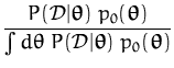
p0(![]() ). Bayes' rule is then used to derive the posterior for
). Bayes' rule is then used to derive the posterior for
![]() :
:
If we are looking for a single value of
![]() , then the most
probable value, the maximum a-posteriori (MAP) estimate of the
parameters is given by maximising the posterior in
eq. (2). The priors over the parameters is the
penalty term added to the cost function, the log-likelihood of the
data, thus the MAP solution is equivalent to the regularisation
framework for solving noisy problems [85,63].
, then the most
probable value, the maximum a-posteriori (MAP) estimate of the
parameters is given by maximising the posterior in
eq. (2). The priors over the parameters is the
penalty term added to the cost function, the log-likelihood of the
data, thus the MAP solution is equivalent to the regularisation
framework for solving noisy problems [85,63].
When using Bayesian methods we are not interested in a single value
for the parameter
![]() but rather the entire probability
distribution. This means that we have to evaluate the normalising
integral from eq. (2) and represent, exactly or
approximately, the whole distribution. The exact representation is
feasible only for a restricted class of models like regression with
Gaussian noise if we assume a Gaussian prior distribution. Generally,
analytical results for the posterior exist only for likelihoods that
are conjugate to the prior distribution [3]. The
exploitation of the full probabilities for general cases requires us
either to sample from the posterior distribution, or to find
appropriate approximations.
but rather the entire probability
distribution. This means that we have to evaluate the normalising
integral from eq. (2) and represent, exactly or
approximately, the whole distribution. The exact representation is
feasible only for a restricted class of models like regression with
Gaussian noise if we assume a Gaussian prior distribution. Generally,
analytical results for the posterior exist only for likelihoods that
are conjugate to the prior distribution [3]. The
exploitation of the full probabilities for general cases requires us
either to sample from the posterior distribution, or to find
appropriate approximations.
Our main interest, irrespective of the model we are using, is in predicting the distribution of the output for an input
x. For
this we have to integrate over the posterior distribution for the
parameter
![]() from eq. (2):
from eq. (2):
The presence of the normalisation integral as in eq. (2), means that computing the predictive distribution is also difficult and we need approximations within the Bayesian framework.
The approximation considered in this thesis is Bayesian online learning [54]. In this learning scheme the approximation to the posterior distribution is found by exploiting the factorising structure of the likelihood in eq. (1): the posterior is built by successive refinement steps, at each step including a single term from the product. These iterations still do not make the posterior tractable, but they can provide efficient approximations in a number of cases.
The online approximation has a particularly appealing structure if we assume both the prior and the posterior distributions for the parameters are Gaussians [55]: online learning retains the mean and covariance of the intractable posterior at each iteration. These statistics are computable for a variety of likelihoods. This simple structure is exploited in applying Bayesian online learning to inference using GPs.
While Bayesian methods provide the posterior probability of the model parameters, the number of parameters and the prior for each parameter is generally fixed in advance. These characteristics cannot be changed during data processing. Consequently, we decide to use GPs which allow us to choose from a larger class of functions whilst retaining the probabilistic treatment.
In Gaussian
processes [5,52,95,100],
instead of specifying the particular parametric model, we encode all
our prior belief about the parameters into a function class
![]()
![]() and the
prior probability of each function drawn from
and the
prior probability of each function drawn from
![]()
![]() . The interest in GPs
from the machine learning community was stimulated by the work of
[49] who showed that using Gaussian prior distributions for
the hidden-to-output weights of a two-layered neural network, in the
limit of infinitely many hidden neurons and a correspondingly scaled
prior variances, is equivalent to a Gaussian process. The advantage
of the functional specification (GPs) over the parametric one (neural
networks) is that usually the function class is larger, giving us more
flexibility in modelling, whilst over-fitting is avoided using the
Bayesian framework.
. The interest in GPs
from the machine learning community was stimulated by the work of
[49] who showed that using Gaussian prior distributions for
the hidden-to-output weights of a two-layered neural network, in the
limit of infinitely many hidden neurons and a correspondingly scaled
prior variances, is equivalent to a Gaussian process. The advantage
of the functional specification (GPs) over the parametric one (neural
networks) is that usually the function class is larger, giving us more
flexibility in modelling, whilst over-fitting is avoided using the
Bayesian framework.
Probabilities for functions are translated to probabilities for random
variables using a finite sample from the function at input positions
![]() = {x1,...,xN}. GPs assign to each
x from the
input set a random variable
fx. The joint distribution of the
random variables
f
= {x1,...,xN}. GPs assign to each
x from the
input set a random variable
fx. The joint distribution of the
random variables
f![]() = [f (x1),..., f (xN)]T is
Gaussian:
= [f (x1),..., f (xN)]T is
Gaussian:
with
K0 = {K0(xi,xj)}ij = 1N the positive definite
covariance matrix and
![]() 0 = [
0 = [![]() (x1),...,
(x1),...,![]() (xN)]T is
the mean function given a-priori. The function generating the
covariance matrix is the positive definite kernel function: the matrix
K0 is a positive definite matrix for any choice of the input set
(xN)]T is
the mean function given a-priori. The function generating the
covariance matrix is the positive definite kernel function: the matrix
K0 is a positive definite matrix for any choice of the input set
![]() .
.
To use GPs for inference, we condition the data likelihood on the GP
as
P(y|x, fx). Bayesian inference for the posterior
process can be written similarly to the parametric case in
eq. (2) from the previous section using the set of
training inputs ![]() . The predictive distribution for an unseen
input
x, as in eq. (3) is:
. The predictive distribution for an unseen
input
x, as in eq. (3) is:
where
p0(fx,f![]() ) is the joint Gaussian distribution of the
random variables at the training and test locations, and
marginalisation is done only with respect to
f
) is the joint Gaussian distribution of the
random variables at the training and test locations, and
marginalisation is done only with respect to
f![]() .
.
From the predictive distribution we see the problems we have to address when GP inference is used in practise:
Both problems are a result of the non-parametric nature of GPs: the ``parameters'' to be learnt are the continuous mean and covariance functions which describe fx. To solve these problems, in this thesis we propose:
Since we use GPs that are non-parametric, we expect that the number of
our parameters will scale with the size of the data set. This scaling
is obvious if we consider the MAP solution to the posterior of
eq. (2) given by the representer theorem
of [40] (generalised by [72]):
for any log-likelihood function, the maximiser of the posterior
eq. (2) is given in terms of a linear combination of
kernel functions
K0(x,x![]() ) centred at the data points:
) centred at the data points:
The importance of the representer theorem is that the solution
![]() (x) is given by the set of coefficients
(x) is given by the set of coefficients
![]() = [
= [![]() ]T that are independent of the input
x at
which the value of the function is estimated. This theorem is the
basis for the successful applications of the kernel
methods [77,71] and support vector machines
(SVMs) [93].
]T that are independent of the input
x at
which the value of the function is estimated. This theorem is the
basis for the successful applications of the kernel
methods [77,71] and support vector machines
(SVMs) [93].
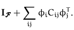
From a Bayesian perspective, the drawback of the representer theorem is that it does not provide probabilistic estimates. Using the Bayesian framework, in Chapter 2 we give a parametrisation lemma that is similar to the representer theorem and provides a representation of the moments of the posterior GP. It is shown that the moments can be expressed, similarly to eq. (6), using combinations of the kernel function. For the first moment the parametrisation has the form given by the representer theorem, and additionally to eq. (6), we have the posterior kernel as:
with ``parameter'' matrix C = {Cij} specifying the posterior kernel function. Estimation of the posterior kernel leads directly to estimating the uncertainty when making predictions. We consider approximations to the posterior process by keeping only the first two moments. Thus the representation lemma provides the parameters that represent the GP approximation to the posterior process.
We can use now GPs as a latent process which will be approximated during learning. Predictions are based on the marginalisation of the approximated posterior process. If we assume factorising likelihoods, the prediction for x will only involve a single Gaussian random variable fx and combining with the likelihood function, requiring a one-dimensional integral.
Approximating the underlying GP allows the modeller to assess the uncertainty of the predictions using Bayesian confidence intervals in the regression case, or to estimate the posterior class probabilities for classification. It also opens the possibility to treat other nonstandard data models like density modelling (Section 5.3) or inference of wind-fields [48,2]) using GPs (Section 5.4). The GP approximation of the posterior process also allows the estimation of the marginal likelihood, leading to model selection. Although it is important, the model selection is not discussed in this thesis, being an area of further research.
The MAP solution of eq. (6) provides an intuitive understanding of kernel algorithms and SVMs: to increase the degrees of freedom in these algorithms the inputs are first projected into a high-dimensional feature space. A simple, usually linear, algorithm is employed therein to obtain the results.
The key element of the design of such algorithms is that the results are written using only the scalar product between the feature space images of the inputs, thus the explicit projection into the feature space is never needed. The scalar products are replaced with a bivariate function, the kernel function of the GP; this way the feature space associated to a particular kernel need not even be finite-dimensional (e.g. the feature space associated with an RBF kernel). This procedure of ``kernelising'' linear algorithms was frequently applied and the over-fitting due to the increased flexibility of the model was avoided by considering penalties on model complexity. The classical example of using kernels is for classification [93]: the Support Vector Machines (SVMs).
To illustrate the relation between the kernel function and the feature
spaces, we use the eigen-decomposition of the kernel function
K0(x,x![]() )
)
with
![]() (x) are the eigenfunctions of the kernel and
(x) are the eigenfunctions of the kernel and
![]() are the eigenvalues corresponding to
are the eigenvalues corresponding to
![]() (x). The
kernel functions need to be positive definite, meaning that the
summation is over a countable number of functions and
(x). The
kernel functions need to be positive definite, meaning that the
summation is over a countable number of functions and
![]() > 0 [45] (or e.g. in [92]). Grouping
the rescaled functions
> 0 [45] (or e.g. in [92]). Grouping
the rescaled functions
![]()
![]() (x) in a vector
denoted
(x) in a vector
denoted
![]() leads to a space of features into which each input
x is projected. We will use
leads to a space of features into which each input
x is projected. We will use
![]() to denote the feature space and
to denote the feature space and
![]() will be the image of
x.
will be the image of
x.
Using the feature space
![]()
![]() , the kernel function
K0(x,x
, the kernel function
K0(x,x![]() )
becomes a scalar product in the Euclidean feature space and
eq. (8) is rewritten as:
)
becomes a scalar product in the Euclidean feature space and
eq. (8) is rewritten as:
With scalar products replacing the kernel functions in
eq. (6), the MAP solution of the representer theorem
is a scalar product between
![]() , the feature space image of the
input and the MAP solution, an element of the feature space,
written as in eq. (10). In
Section 2.3.1 we show that the parametrisation lemma
for GPs implies that the approximated posterior process is a normal distributions in the feature space
, the feature space image of the
input and the MAP solution, an element of the feature space,
written as in eq. (10). In
Section 2.3.1 we show that the parametrisation lemma
for GPs implies that the approximated posterior process is a normal distributions in the feature space
![]()
![]() with mean and covariance
with mean and covariance
where
![]() is the unit matrix, the prior distribution of the
parameters in the feature space. The equivalence of the GPs with the
normal distributions is explored in the thesis. Similarly to the
design of kernel algorithms, we consider the fictitious feature space
and the normal distribution of the parameters and express various
quantities in terms of the kernel function and the parameters of the
normal distribution.
is the unit matrix, the prior distribution of the
parameters in the feature space. The equivalence of the GPs with the
normal distributions is explored in the thesis. Similarly to the
design of kernel algorithms, we consider the fictitious feature space
and the normal distribution of the parameters and express various
quantities in terms of the kernel function and the parameters of the
normal distribution.
The parametrisation lemma provides the approximated posterior process
using the parameters ![]() and Cij, solving the problem of
representing the functional entity concisely.
and Cij, solving the problem of
representing the functional entity concisely.
A different issue, faced when implementing GP inference in practise,
is the increasing number of parameters as the data size grows. For
non-probabilistic kernel machines the scaling is linear: we need to
store only ![]() . When computing these parameters, however, we
need the whole kernel matrix and usually inversions for these
matrices. This makes kernel methods computationally infeasible for
large datasets: the time required to compute a general matrix
inversion grows as N3. The time requirement for GPs given by the
parametrisation lemma is also cubic in the number of data points,
resulting in the same limitation as the other kernel methods.
. When computing these parameters, however, we
need the whole kernel matrix and usually inversions for these
matrices. This makes kernel methods computationally infeasible for
large datasets: the time required to compute a general matrix
inversion grows as N3. The time requirement for GPs given by the
parametrisation lemma is also cubic in the number of data points,
resulting in the same limitation as the other kernel methods.
The main contribution of this thesis is to provide a framework for a sparse parametrisation of GPs. The reduction of parameters is achieved by retaining only a subset of the inputs in the expressions of the posterior mean and kernel functions. This is achieved by minimising a distance between two GPs parametrised using a small number of basis vectors. Basis vectors in this thesis denote the input data that are retained in the sums of eqs. (6) and (7) after the algorithm finished.
In Chapter 3 sparsity is combined with the Bayesian
online learning to produce an efficient algorithm to infer the latent
GP. The learning rules are such that the size of the basis vector set
can be set in advance and the computing time is reduced to linear with
respect to the data size:
![]() (Np2) with p the cardinality of
the basis vector set.
(Np2) with p the cardinality of
the basis vector set.
The sparse solution is similar to the result of the popular SVMs that also obtain an expansion of the result using a small set of support vectors. To get sparse solutions, in SVMs we need to solve a quadratic optimisation problem involving the whole data set, irrespective how sparse the final solutions are. In this thesis the iterative online algorithm eliminates the need to solve this demanding problem, reducing the computational requirement.
The framework for sparsity does not make assumptions about the likelihood of the problem, thus the resulting algorithm is a general one, applicable for a large class of likelihoods.
The thesis is organised as follows:
The details of calculations, to preserve the flow of the main ideas, are put in appendices.
We use bold lowercase letters for vectors and bold uppercase for
matrices. Scalar quantities will be typeset in normal, such as the
particular elements of a vector or matrix, thus a vector
![]() = [
= [![]() ,
,![]() ,...,
,...,![]() ]T is a d-dimensional
vector with corresponding components.
]T is a d-dimensional
vector with corresponding components.
We summarise the notation in the thesis: