Important: some text is copy-pasted from the
thesis
(see References). For more compact information you can look at the
Neural Computation article.
Examples of Online Gaussian Process Inference
Online inference is applicable whenever one can compute the
local posterior mean and (co)variance. The term local refers
to the current example and a previous approximation to the posterior
process.
An equivalent formulation is to obtain analytically the averaged
likelihod for the current input.
The update coefficients are obtained by differentiating its
logarithm.
It is important that the average needed for the posterior process to
be implemented is one-dimensional (or two, but definitely does not
scale with the number of examples as with the normal use of GP
inference).
In all situations below we compute the scalar
coefficients based on the following relation:

|
(53)
|
The brackects within the logarithm denote averaging with respect to a
Gaussian ft+1-- average for which
there often exist good approximations (lookup-tables, or efficient
numerical solutions).
In the examples that follow different likelihoods are presented. It
is emphasised that the only difference is the
likelihood, since
the desscription of the estimation procedure will not be repeated.
-
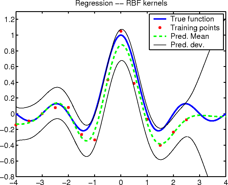
A trivial example of the above pocedure is regression with
additive Gaussian noise assumption. The image below shows the
resulting mean of the posterior process together with the true
function and the predicted variance arond the mean.
(click here to see the explanatory section from the thesis)
-
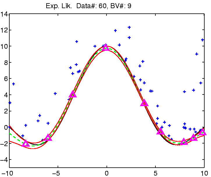
There are cases when normal noise assumption is inappropriate:
the noise is e.g. Gaussian, or its type is not known but there
is the possibility of having outliers in the data. Applying the
Gaussian likelihood would deter the performance of the GP
inference (inappropriate prior knowledge).
The figure below shows such a situation where the known noise is
not Gaussian, but a heavy-tailed exponential and additionally we
also know that it is only positive. The green line shows the posterior
approximation and the pair of red lines
are the Bayesian confidence intervals around the
posterior mean.
A PDF version of the link is available
HERE.
(click here to go to the Robust Regression section)
-
Classification is not tractable analytically. Using the online
procedure we obtain powerful approximations to the posterior
process.
Click to go to the related link.
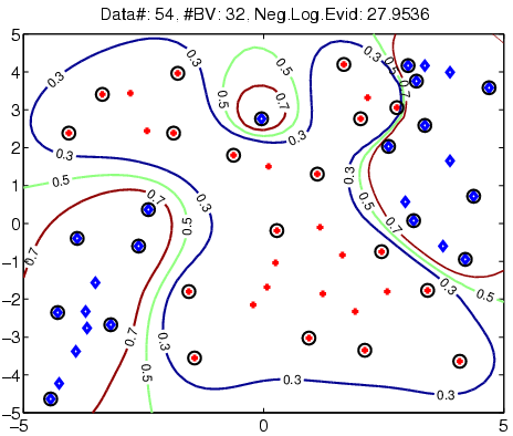
The figure illustrates the OGP classification on a toy
two-dimensional example. The red/blue symbols are the labelled
inputs, the black circles over the inputs show the location of
the Basis Vectors. The contour lines show the
approximated posterior class-conditional probability, which can
be translated into class boundary (0.5,
green), and confidence regions (brown and blue
lines).
-
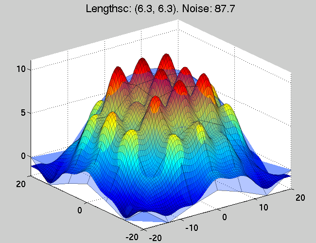
Inferring wind-fields from remote observations poses two issues
that need to be tackled: the first one is to represent
two-dimensional Gaussian fields, or processes (for each location
we have random variables specifying the X-, and
Y-directions.
The second problem is the inference with the inherently
non-tractable likelihood model, governed by the underlying
physics governing the wave formation and light reflection from
water surfaces.
(click to go to the relevant section)

-
Transductive learning is used whenever one wants to use the
information about the location of the future test points. The
likelihood model Gaussian regression, thus the novelty of this
type of learning is the inclusion of the special information
about the test points.
A PDF version of the link is available
HERE.
(click here to go to the Transductive Learning section)
Questions, comments, suggestions: contact Lehel
Csató.