Data Assimilation with sparse GPs
Inferring wind-fields from remote observations poses two issues that
need to be tackled: the first one is to represent two-dimensional
Gaussian fields, or processes (for each location we have random
variables specifying the X-, and
Y-directions.
The second problem is the inference with the inherently non-tractable
likelihood model, governed by the underlying physics governing the
wave formation and light reflection from water surfaces.
Inference with Vector Gaussian processes
Due to the pair of Gaussian random variables z at each
location, the kernel function
W0(x,y) is a 2×2 matrix, specifying
the pairwise cross-correlation between the components at different
spatial positions (notice that the notation of the kernel function is
different). In the following
z denotes the random vector
corresponding to the wind-field at a single position and
where
 =
[z1,...,zN]T denotes the
concatenation of the local wind field components
zi. These components are random variables
corresponding to a spatial location
xi. These locations specify the prior covariance
matrix for the vector
,
given by
W0 =
{W0(xi,xj)}ij
= 1N. The two-dimensional Gaussian
p0 is the prior GP marginalised at
zi, with zero-mean and covariance
W0i.
=
[z1,...,zN]T denotes the
concatenation of the local wind field components
zi. These components are random variables
corresponding to a spatial location
xi. These locations specify the prior covariance
matrix for the vector
,
given by
W0 =
{W0(xi,xj)}ij
= 1N. The two-dimensional Gaussian
p0 is the prior GP marginalised at
zi, with zero-mean and covariance
W0i.
In order to have a global model from the N, we combine them
with a zero-mean vector GP [13,47]:
where si is the vector of local observations
at spatial location xi and
zi is the corresponding vector of random variables.
The representation of the posterior GP
thus requires vector quantities: the marginal of the vector GP at a
spatial location
x (and
y for the covariance)
has a bivariate Gaussian distribution with mean and covariance
function of
zx 
 2
2 represented as:

|
(170) |
where
 z(1),z(2),...,z(N) and
{Cz(ij)}i, j = 1, N are the
coefficients of the vector GP describing the posterior mean and
variance respectively. Although technical details, the quantities in
are not scalars, one has to ``re-shuffle'' the expression in
eq. (170).
z(1),z(2),...,z(N) and
{Cz(ij)}i, j = 1, N are the
coefficients of the vector GP describing the posterior mean and
variance respectively. Although technical details, the quantities in
are not scalars, one has to ``re-shuffle'' the expression in
eq. (170).
Notice that this is exactly the same representation as for
the scalar random variables, but due to the coupling in the likelihood
model we have coupling in the representation of the posterior also.
Again, as with other likelihood models, in order to have a
representation to the posterior, one has to compute the average of the
likelihood p(si|zi). The
different methods of performing the inference are detailed next.
Dealing with the likelihood
The likelihood is complex non-Gaussian and non-linearly dependent of
the wind-direction. In the simplest case we assume that the
scatterometer reads the output of a known nonlinear
transformation but this output is corrupted by non-gaussian noise.
Either the nonlinearity or the non-gaussianity make the posterior
process non-tractable analytically. We present methods to
approximate this non-tractable model.
Local inverse model:
Instead of using the direct likelihood
p(si|zi), we transform
eq. (170) using Bayes theorem to
obtain the following expression for the posterior:
where a mixture density network (MDN) [
4] is used to model the
conditional dependence of the local wind vector
zi = (
ui,
vi) on
the local scatterometer observations
si:
pm(zi|si, ) = ) =    (zi|cij, (zi|cij, ) )
|
(168) |
where
 is the union of the MDN parameters: for each
observation at location
xi we have the weightings
is the union of the MDN parameters: for each
observation at location
xi we have the weightings
 for the local Gaussians
 (cij,
(cij, )
where
cij is the mean and
is the variance. The parameters of the MDN
are determined using an independent training set [22] and are considered known
in this section.
The prior GP, which also has a set of hyper-parameters, was tuned
carefully to represent features seen in real wind fields and is also
known here.
)
where
cij is the mean and
is the variance. The parameters of the MDN
are determined using an independent training set [22] and are considered known
in this section.
The prior GP, which also has a set of hyper-parameters, was tuned
carefully to represent features seen in real wind fields and is also
known here.
Forward models
Here the forward wind-field to scatterometer mapping was
learned using a truncated Fourier series for the scatterometer values
and the coefficients of the Fourier series were the outputs of RBF
networks whose inputs are the relative wind direction (to the
satellite) and the incidence angle.
A gaussian noise model was assumed and a Taylor expansion of the RBF
networks has been made, obtaining an approximation to the log-average.
The problem with this model is that it does not have a meaningful
approximation for low wind-speeds, thus there has to be an
initial small wind-direction.
Sampling from the local posterior
This approach also used the inferred Fourier series about the forward
models from batch training, but rather than doing a Taylor expansion
of the RBF functions in the likelihood, it used importance sampling
instead.
The update coefficients were computed from the sampling mean and
covariances of the resulting local posterior approximation.
Results
The results of the above methods were roughly similar, but their
stability was different. Due to the local symmetries present in the
model -- opposite wind-fields tend to produce very similar waves --
there are several local minima in which the inference can get trapped.
The forward model, if used with a zero-mean prior Gaussian process,
gave inconsistent solutions, thus several restarts were needed. The
solutions of the remaining two models were fairly consistent.
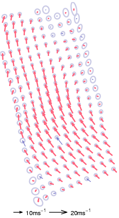
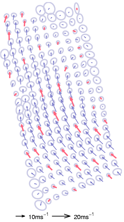
Figure 1. The results of the direct inverse model. The left
sub-figure shows the inference when the GP representation was kept
intact (189 in this case) and this is to be contrasted with
the right sub-figure where only 38 BVs gave the same
mean function, but with higher posterior uncertainty, illustrated
with larger ellipses.
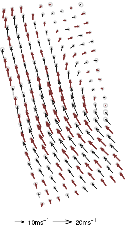
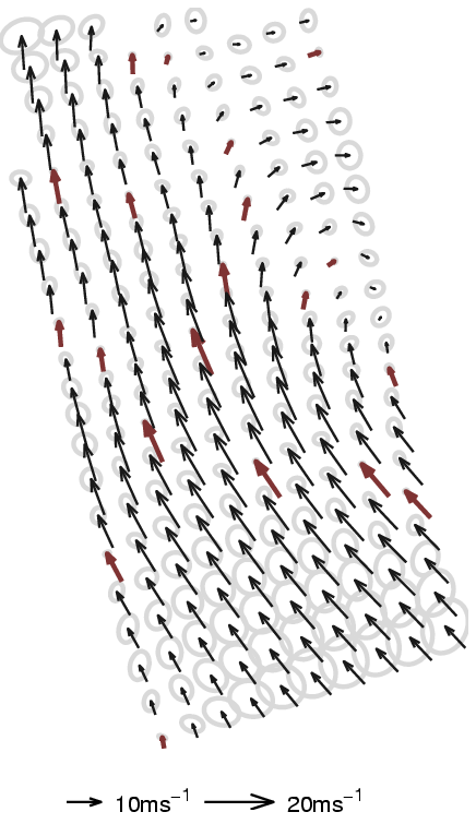
Figure 2. Results from the same data using the sampling
procedure (different colour coding). The left sub-figure shows the
inference with a high number of BVs (100) whilst there are
only 20 BVs kept to represent the posterior GP. As in the
previous case, the uncertainties corresponding to a spatial location
is illustrated using ellipses.
Problems
The plots below show the problems one can encounter if using sampling
to obtain the update coefficients.
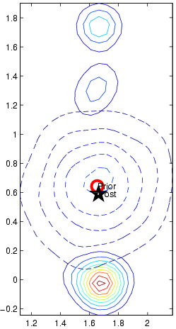
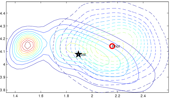
Figure 3. Contour plots of the local Gaussian prior (dashed
line) and the posterior computed using importance sampling. We see
that the variance along the Y-axis is very elongated, much
longer than the associated prior distribution. The iterative
approximation trimmed the long tail of the posterior to that of the prior, keeping the inference numerically stable.
-
Bullen R.J, Cornford D, Nabney I.T. (2003): Outlier Detection in
Scatterometer Data: Neural Network Approaches, Neural
Networks, 16, 3-4, 419--426.
-
Cornford D, Csato L, Evans D.J, Opper M. (2003): Bayesian analysis
of the scatterometer wind-retrieval problem: some new approaches,
Submitted to the Royal statistical Society, a draft
version is available: in Postscript:
jrss02.ps.gz and in PDF format:
jrss02.pdf.
-
Csato L, Cornford D, Opper M. (2001): Online Approximations for
Wind-Field Models, In International Conference on Neural
Networks ICANN 2001, draft version available from the NCRG repository.
The PDF version of this document can be found here.
Questions, comments, suggestions: contact Lehel
Csató.
