The Acrobat file for the whole document is HERE.

Transductive learning

In classical machine learning the result of the inference relies only on the training set and it is always independent of the test set. Whilst statistically sound and reasonable, many applications have a large number of unlabeled input which cannot be used in training, as for example in chemical or biological areas where there is a plethora of experimental result but labelling them -- or giving a ``desired value'' for an experimental outcome is very expensive and time-consuming (this type of problem is tackled in active learning).

In transductive learning the situation, from the machine learning point of view is simpler, but similar: all unlabeled points belong to the test set. This means additional information for the learning algorithm that needs to be exploited and it can be particularly important for nonparametric methods: the performance of the sparse inference using a subset of the training inputs can significantly vary as a function of the location of the subset (Basis-, Support- or Relevance- Vector set) on which the approximation is based.

The inclusion of this special knowledge within the GP inference scheme was recently presented in Schwaighofer, Tresp (2003). The inference using this special knowledge is called query learning and the query points are merely a different name for the test points.

The methodology proposed here is similar to the above method: the set of Basis Vectors is fixed a-priori to the set of query points. The GP is initialised with the query set but no training output data, accomplished by a constant likelihood. We can then perform pseudo-learning to learn the locations of the query points - remember that the associated GP, although having a different representation, is still the prior process.

Having this modified representation for the prior process, we can iterate the sparse learning which first projects the GP to the set of Basis Vectors (which is the query set). The BV set is unaltered during learning.

In the following a MATLAB code is presented that learns the two-dimensional sinc function f(x,y)=sin(r)/r where r is the radius of the two-dimensional input in polar coordinates. The function is available within the OGP package, named demogp_fixed (uses a fixed BV set).

Fig.1 below shows the location of the training set (smaller black 'x' signs) and the Basis Vectors which is also the query set. On Fig.2 one sees the result of the OGP inference using the query set. Note that due to the (in this case purposeful) mismatch of model parameters and the function to be approximated, the approximation is quite poor.

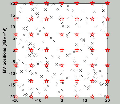
Location of the training and query inputs

Figure 1. The location of the (200) training data and the (49) query points.

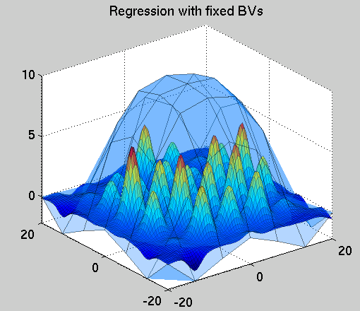
Approximation performance without hyper-parameter adaptation

Figure 2. The initial result of the inference using the predefined set of hyperparameters. It can be seen that the fit at the training locations is not particularly good, since the GP cares now only about the query point locations, placed on a 7x7 rectangular grid. The semi-transparent cover is the function to pe approximated and the surface with the local humps is the actual approximator.

Further on, as the hyperparameters are better fitted to the function, the approximation via transductive learning becomes better. This is visualised on Figs. 3 and 4. The algorithm automatically detects that the smoothness of the function allows an even sparser representation and many elements of the query set are removed (they are redundant), as can be seen from comparing the initial configuration from Fig. 1 with that of Fig. 5. The Matlab code is explained in the Section following the figures.

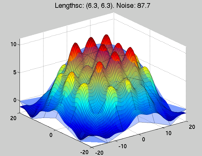
Approximation performance after single hyper-parameter optimisation

Figure 3. The function approximation after a single hyper-parameter optimisation step -- an optimisation procedure of the marginal likelihood. It can be seen that the approximation now is much better - this is due to the better fit of the GP lengthscale parameters to the function.

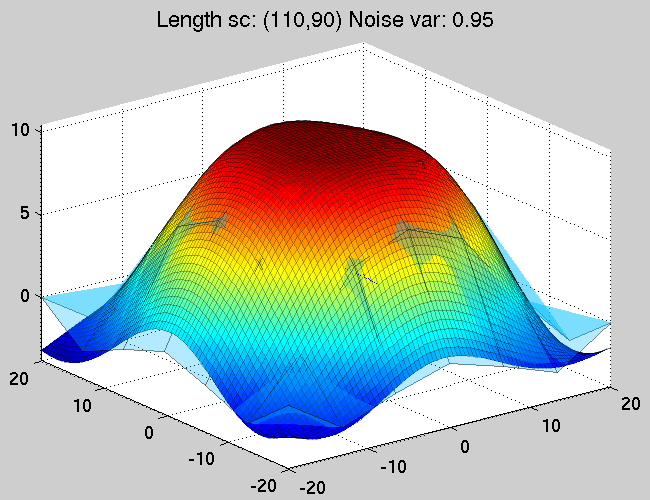
Approximation performance after 5 hyper-parameter optimisations

Figure 4. The approximating and the true funtions after 5 steps of iterating between the optimisation of the GP parameters with fixed hyperparameters and optimising the hyperparameters whilst keeping the GP parameters fixed.

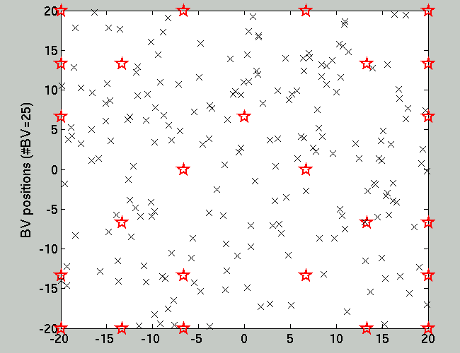
Figure 5. Since the surface of the function to be approximated is smooth, there are no need for that many Basis Vectors. The final configuration of the OGP structure includes only 25 elements (sampling or computation with fewer Basis Vectors is faster). Yet it is clear that the approximation performance is not affected.

Matlab code

The matlab file, provided in the code section of these pages, is named demogp_fixed.m.

We first declare to global variables we are going to use


global net gpopt ep

The next step is to declare variables related to the data generation process:

sig02   = 0.3;	              % noise variance
nType   = 'gauss';            % noise TYPE
nTest   = 49;                 % TEST set size = BV SET size
nTrain  = 200;                % TRAINING set size
gX      = [-20:0.5:20];
gN      = length(gX);
[pX pY] = meshgrid(gX);
pX      = [pX(:) pY(:)];

Then the training and test datasets are generated:

% training points are randomly placed
[xTrain, yTrain] = sinc2data(nType,nTrain,sig02,[],0,20,20);
% test points are on a grid
[xTest,  yTest]  = sinc2data(nType,nTest,0,[],1,20,20);

We initialise the OGP structure. The first function is similar to a "constructor", the second function specifies the likelihood we are using, then the threshold value thresh - for numerical stability - is set.

ogp(2,1, ...                  % input/output dimension
    'sqexp', ...              % kernel type
    [1/[2 2] 3 0]);           % kernel parameters

ogpinit(@c_reg_gauss,...
        0.5, ...              % initial value for the lik. par.
        @em_gauss);           % function to adjust lik. noise
net.thresh    = 1e-1;         % the admission threshold for new BVs
% SAVING
netS = net;

The next two lines set up the transductive- or query learning: we initialise the BV-s of the OGP structure with the test set locations.

% SETTING the initial OGP structure
net = netS;
% FIXED BV set
ogpemptybv(xTest(randperm(size(xTest,1)),:));
net.isBVfixed = 1;

Code that controls the various parameters that will be displayed during learning (not really important).

% What to print out during learning
gpopt = defoptions;           % default values
gpopt.pavg  = 1;              % log-average
gpopt.ptest = 1;              % test error
gpopt.xtest = xTest;          % the test inputs
gpopt.ytest = yTest;          % desired outputs
gpopt.disperr=0;
gpopt.freq  = 10;             % frequency of measuring the errors
gpopt.postopt.isep  = 1;      % USING the TAP/EP algorithm
gpopt.postopt.itn   = 3;      % number of EP iteration with CHANGING BVs
gpopt.postopt.fixitn= 2;      % FIXING the BV set.

The sequence of training and hyper-parameter estimation.

for iHyp=1:5;

  ogptrain(xTrain,yTrain);

  ogpreset;

  fixErr(bInd,:) = gpopt.testerror;
end;

and the rest of the code involves plotting and visualisation (not explained here, see demogp_fixed for details)

References

The source code - Matlab file - of the code is named demogp_fixed.m and is included in the package.
Kernel Machines: Links and references to/about Kernel methods. Has several good tutorials presenting the Support Vector Machines. Web location: www.kernel-machines.org.
Schwaighofer A, Tresp V (2003): Transductive and inductive methods for approximate Gaussian process regression. In Becker S, Thrun S, Obermayer K (ed): Advances in Neural Information Processing Systems 15. MIT Press, 2003.

Questions, comments, suggestions: contact Lehel Csató.