Glossary of terms
- Gaussian Process:
- Stochastic process with only two nontrivial (nonzero) moments. A
stochastic process is a collection of random variables indexed with
arbitrary indices. The index set can be of any cardinality:
finite - the case of an alphabet; countably infinite - the natural
numbers; the time axis; or the d-dimensional Euclidean space. For
Gaussian processes any finite realisation (ie. collection of random
variables corresponding to an index set) has a joint Gaussian
distribution.
To sample from a Gaussian process first we have to set the locations
associated with the collection of random variables, e.g. a regular
grid over a domain. Given the locations, one generates then the mean
function and the covariance matrix and samples using that covariance
matrix.
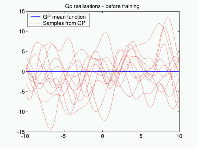
The figure below shows samples from a GP with zero mean function
(blue thick line). Each line is a single sample and the
histograms at each (horizontal) X-location over many samples should
look like Gaussians.
In GP inference (usually zero-mean) GPs are used as priors and the
combination with the data - specified via likelihood function -
leads to a posterior process.
- Prior distribution
- Specifies the prior belief of the range the model
parameters have. In non-parametric case the prior is over the random
functions and beliefs are usually only smoothness assumptions
encoded in the kernel function .
- Likelihood function
- It is a probabilistic formulation of the cost-, or loss
function. Most cost functions (with some notable exceptions, like the
epsilon-loss for classification) have a corresponding representation
using likelihoods, eg. the quadratic loss corresponds to the Gaussian
likelihood.
- Bayesian inference
- Probabilistic inference that computes the distribution
of the model parameters and gives prediction for previously unseen
input values probabilistically. To perform the inference we need a prior distribution for the parameters and a likelihood function for the data set at hand.
One computes the posterior distribution of
the parameters by combining the prior and the likelihood using Bayes'
rule. In Bayesian inference for non-parametric models, after
choosing a prior over a suitable function space or a prior process,
one obtains a posterior distribution over the same function
space.
- Posterior process
- Ideally the whole posterior process should be used to perform
inference for unseen data, however this is impossible either due to
intractability of the posterior process or the large memory
requirement required for the exact posterior process.
In the framework of sparse online GPs the
intractability is dealt with using GP approximations to the true
posterior, and the increasing memory requirements are solved using
sparsity and retaining only a small subset of the inputs to
represent the GPs.
The following figure plots the inferred GP from noisy samples of the
sinc function: sin(x)/x . The model parameters were deliberately
chosen so that the fit is not good.
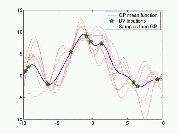
- Basis Vector set (BV)
- Stores the input locations used to represent the GP. In the
figure above the green stars on the mean function indicate the
BVs. More BVs mean more accurate representation of the posterior
process but at the same time more computational time
(scaling is cubic with respect to BV set size).
- Kernel functions
- Two-argument functions which tell the covariance between two
random variables located at the arguments of the functions. The
kernel function is the generator of the covariance matrix for any
collection of random variables sampled from a GP. In the family of kernel methods
the kernel function is used as a basis for the result: the regressor
function is obtained as linear combination of the kernel
function with one of the arguments fixed to the position of the
input point. One of the most often used kernel function if the
Radial Basis Function Kernel (see any review).
Questions, comments, suggestions: contact Lehel
Csató.