Important: since it is quite technical, the text is mainly
copy-pasted from the
thesis (see
References). For more compact information you can look at the
Neural Computation article.
Sparsity in Gaussian Processes
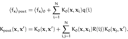
Let us recall the parametrisation of the posterior moments (
Lemma 3.1 in the GP representation)
which states that
whatever the likelihood, given finite data
sample, the moments of the posterior can be expressed as a
linear/bilinear (multilinear if one wants posterior moments of higher
order) combination of the prior kernel function:
|
(33)
|
where
K0(xl,xm)
is the prior kernel and N is the number of input data.
However, we want to save resources and approximate the large sum with
a more compact representation of the approximated posterior GP. A
sequential selection procedure to build a set of
``basis
vectors'', or

set, is provided.
The tool to obtain the sparse representation is the computation of the
KL-distance between two GPs obtained
from the same prior
GP0 (details can be found in the
Thesis at Section
3.2. The KL-distance is
computed using the equivalence of the GPs with the normal distribution
in the feature space induced by the kernel.
The Kullback-Leibler divergence
Let us denote the feature space induced by the kernel with

and let the mean and covariance of the two GPs (again, Gaussian random
variables in the feature space
) be
(
 1
1,
 1
1
)
and
(
2,
2
)
respectively. The KL-distance can then be written as:
2KL( 1|2)
= (
2
-
1)T2-1(2
-
1)
+ tr 1|2)
= (
2
-
1)T2-1(2
-
1)
+ tr 12-1 - I 12-1 - I   - ln
- ln 12-1 12-1
|
(66)
|
where the means and the covariances are expressed in the
high-dimensional and unknown feature space
.
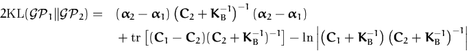
Let us assume that two approximated posterior GPs have the same
set
and denote the kernel Gram matrix of the set with
KB
The two GPs are comppletely specified by their prior kernel and the
distinct set of parameters
(
 1
C1
1
C1)
and
(
2
C2)
This leads to the equation for the KL-distance between two GPs
 . . |
(74) |
where all quantities are those of the dimension of the data (no
feature space involved).
KL-optimal projection
We introduce sparsity by assuming that the GP is a result of some
arbitrary learning algorithm, not
necessarily the online learning from the
Online estimation. This implies that at an arbitrary time
moment
t + 1 we have a set of basis vectors for the GP and the
parameters
t + 1
and
Ct + 1.
We are then looking for the "closest" GP
(

,

)
in the KL-sense (which we know is positive)
with a reduced
set where the last element
xt + 1 has been removed.
This is a constrained optimisation problem with analytically
computable solution.
Rather than (re-) deriving the result of trimming the GP, in
the figure below we provide an intuitive explanation of why the
sparsity works.
Let us focus on the posterior mean, which is a linear combination of
all basis vectors. The
set has
t+1 elements. The single element of the
set is removed which provides the
smallest KL-distance from
the original approximation, intuitively associated with the length of
the residual vector

.
Figure 3.1: Visualisation of the projection. The
last feature vector

is projected to the subspace spanned by
{

,...,

}
resulting in the projection

and its orthogonal residual
.
Since the
real-world data we want to approximate have a
strong structure, he approximations are performant for many examples
(
see the Examples section).
Questions, comments, suggestions: contact Lehel
Csató.
![\includegraphics[]{project.eps}](thesis/img289.png)