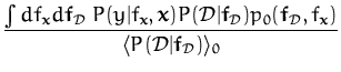
The parametrisation lemma provides us the first two moments of the
posterior process. Apart from the Gaussian regression, where the
results are exact, we can consider the moments of the posterior
process as approximations. This approximation is written in a
data-dependent coordinate system. We are using the feature space
![]()
![]() and the projection
and the projection
![]() of the input
x into
of the input
x into
![]()
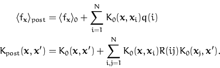
![]() . With the scalar product from
eq. (19)
replacing the kernel function K0, we have the mean
and covariance functions for the posterior process as
. With the scalar product from
eq. (19)
replacing the kernel function K0, we have the mean
and covariance functions for the posterior process as
This shows that the mean function is expressed in the feature space as
a scalar product between two quantities: the feature space image of
x and a ``mean vector''
![]() ,
also a feature-space entity. A similar identification for the
posterior covariance leads to a covariance matrix in the feature space
that fully characterises the covariance function of the posterior
process.
,
also a feature-space entity. A similar identification for the
posterior covariance leads to a covariance matrix in the feature space
that fully characterises the covariance function of the posterior
process.
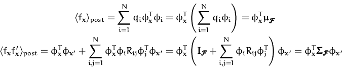
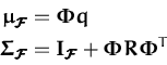
The conclusion is the following: there is a correspondence of the
approximating posterior GP with a Gaussian distribution in the feature
space
![]()
![]() where the mean and the covariance are expressed as
where the mean and the covariance are expressed as
where
![]() is the concatenation of the feature vectors for all data.
is the concatenation of the feature vectors for all data.
This result provides an interpretation of the Bayesian GP inference as a family of Bayesian algorithms performed in a feature space and the result projected back into the input space by expressing it in terms of scalar products. Notice two important additions to the kernel method framework given by the parametrisation lemma:
The main difference between the Bayesian GP learning and the non-Bayesian kernel method framework is that, in contrast to the approaches based on the representer theorem for SVMs which result in a single function, the parametrisation lemma gives a full probabilistic approximation: we are ``projecting'' back the posterior covariance in the input space.
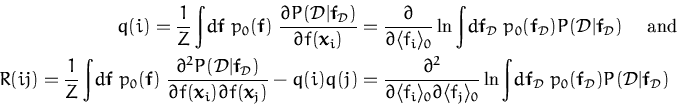
Also an important observation is that the parametrisation is
data-dependent: both the mean and the covariance are expressed in a
coordinate system where the axes are the input vectors ![]() and
q and
R are
coordinates for the mean and covariance respectively. Using once more
the equivalence to the generalised linear models from Section 2.2, the GP approximation
to the posterior GP is a Gaussian approximation to
and
q and
R are
coordinates for the mean and covariance respectively. Using once more
the equivalence to the generalised linear models from Section 2.2, the GP approximation
to the posterior GP is a Gaussian approximation to
![]() .
.
A probabilistic treatment for the regression case has been recently proposed [88] where the probabilistic PCA method [89,67] is extended to the feature space. The PPCA in the kernel space uses a simpler approximation to the covariance which has the form
where the ![]() takes arbitrary values and
W is a diagonal matrix of the size of the data. This
is a special case of the parametrisation lemma of the posterior
GP eq. (48).
This simplification leads to a sparseness. This is the result of an
EM-like algorithm that minimises the KL distance between the empirical
covariance in the feature space
takes arbitrary values and
W is a diagonal matrix of the size of the data. This
is a special case of the parametrisation lemma of the posterior
GP eq. (48).
This simplification leads to a sparseness. This is the result of an
EM-like algorithm that minimises the KL distance between the empirical
covariance in the feature space
![]()
![]()
![]() and the parametrised covariance of eq. (49).
and the parametrised covariance of eq. (49).
In the following the joint normal distribution in the feature space with the data-dependent parametrisation from eq. (48) will be used to deduce the sparsity in the GPs.
Questions, comments, suggestions: contact Lehel Csató.
 ,
,