| Ps(y| ft+1, |
(1) |
The Acrobat file for the whole document is HERE.
Two noise models, exponential but heavy-tailed, are presented. The first noise model has a symmetric Laplace distribution:
where ![]() is the inverse of the noise variance, y is the observed
noisy output, and ft+1 is the latent output which is assumed to be a
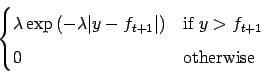
Gaussian random variable. The second model is a non-symmetric version where
the noise can only be positive, thus the likelihood function is:
is the inverse of the noise variance, y is the observed
noisy output, and ft+1 is the latent output which is assumed to be a
Gaussian random variable. The second model is a non-symmetric version where
the noise can only be positive, thus the likelihood function is:
Given a likelihood function and implicitly a training input
![]() , to apply the online learning, we need to compute the
average of this likelihood with respect to a one-dimensional Gaussian
random variable
, to apply the online learning, we need to compute the
average of this likelihood with respect to a one-dimensional Gaussian
random variable
![]() where the Gaussian
distribution is the marginal of the approximated GP at the location of the
new input (see e.g. [4,2]). To obtain the update
coefficients, we then need to compute the derivatives of the log-average
with respect to the prior mean
where the Gaussian
distribution is the marginal of the approximated GP at the location of the
new input (see e.g. [4,2]). To obtain the update
coefficients, we then need to compute the derivatives of the log-average
with respect to the prior mean ![]() .
.
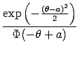
First we compute the average likelihood for the non-symmetric noise model, eq. (2). We define the function g as this average:
where
Note that the pair of parameters
(![]() , a) is enough for parametrising
g since the noise parameter
, a) is enough for parametrising
g since the noise parameter ![]() is fixed in this derivation, Thus,
in the following we will use
g(
is fixed in this derivation, Thus,
in the following we will use
g(![]() , a) and use
, a) and use
![]() f =
f = ![]() f /
f /![]() , result of the definition of
a.
, result of the definition of
a.
We have the update coefficient q(t+1) for the posterior mean function based
on the new data
![]() as:
as:
and similarly one has the updates for the posterior kernel rt+1 as
where
 = =   |
When applying online learning, we iterate over the inputs
![]() , at time t < N having an estimate of the
GP marginal as a normal distribution
, at time t < N having an estimate of the
GP marginal as a normal distribution
![]() and
computing
(q(t+1), r(t+1)) based on eqs. (5)
and (6).
and
computing
(q(t+1), r(t+1)) based on eqs. (5)
and (6).
The update coefficients for the symmetric noise are obtained similarly to the positive case, based on the following averaged likelihood:
Repeating the deduction from the positive noise case, we have the first and
second derivatives as
| q(t+1) | = | 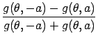 |
|
| r(t+1) | = |  exp exp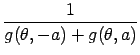 |
The above equations need to estimate the logarithm of the error function
(
![]() ), which can be very unstable. In coding the Matlab implementation of
the robust regression, an asymptotic expansion was used whenever the direct
estimation of the
), which can be very unstable. In coding the Matlab implementation of
the robust regression, an asymptotic expansion was used whenever the direct
estimation of the
![]() function became numerically unstable. See the
Matlab code for details [3].
function became numerically unstable. See the
Matlab code for details [3].
Since all models are exponential, we can adapt the likelihood parameters. This is a multi-step procedure and it takes place after the online iterations: it assumes that there is an approximation to the posterior GP (obtained with fixed likelihood parameters). This is the E-step from the EM algorithm [1,5].
In the M-step we maximise the following lower-bound to the marginal likelihood (model evidence):
which again involves only one-dimensional integrals (i.i.d. data were
assumed), which leads to the following values for the likelihood parameters:
| = | |||
| = |
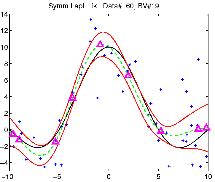
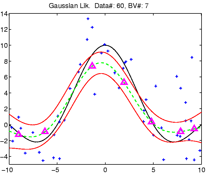
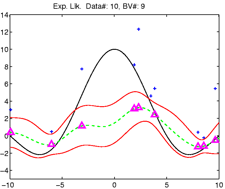
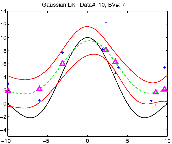
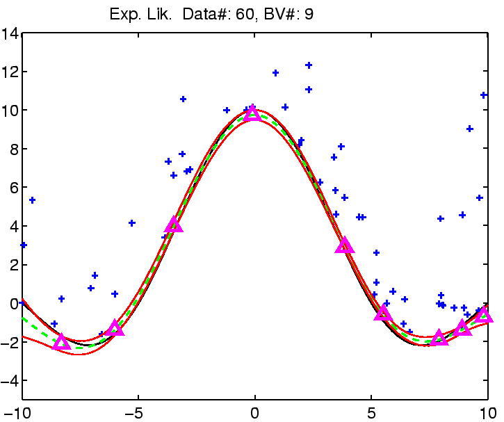
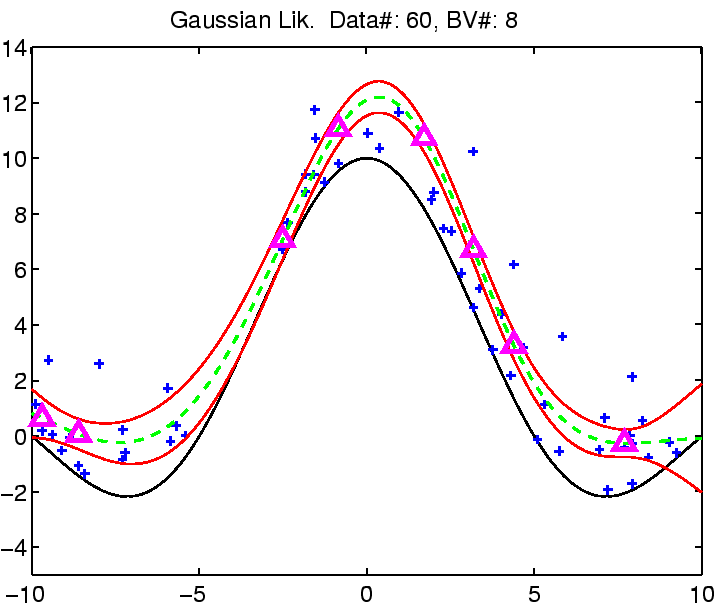
In the following the regression with robust models is demonstrated on
a toy example: the estimation of the noisy
![]() function.
function.
The estimation was compared with Gaussian noise assumption, thus involving three models for the likelihood function for which we can estimate the noise (see the EM algorithm from the previous section). See figure captions for more explanation.
|
|
| (a) | (b) |
|
|
| (a) | (b) |
|
|
| (c) | (d) |
Questions, comments, suggestions: contact Lehel Csató.
 ,
, 
 -
-