Important: since it is quite technical, some text is mainly
copy-pasted from the
thesis (see
References). For more compact information you can look at the
Neural Computation article.
Sparse OGP Classification
Binary classification is not tractable analytically. But if on uses
the probit model [
49]
where a binary value
y 
{ - 1, 1} is assigned to an input
x  m
m with the data likelihood
where

is the noise variance and

is the cumulative Gaussian
distribution:
The shape of this likelihood resembles a
sigmoidal, the main benefit of this choice is that its average with
respect to a Gaussian measure is computable. We can compute the
predictive distribution at a new example
x:
p(y|x, ,C) = ,C) =  P(y|fx) P(y|fx) = Erf = Erf  
|
(144) |
where
 fx
fx
=
kxT
is the mean of the GP at
x and

=

+
k*x +
kxTCkx.
It is the predictive distribution of the new data, that is the
Gaussian average of an other Gaussian. The result is obtained by
changing the order of integrands in the Bayesian predictive
distribution eq. (
143) and back-substituting
the definition of the error function.
Based on eq. (
53), for a given
input-output pair
(
x,
y) the update coefficients
q(t +
1) and
r(t + 1) are computed by
differentiating the logarithm of the averaged likelihood from
eq. (
145) with
respect to the mean at
xt + 1 [
17]:
q(t + 1) =   r(t + 1) = r(t + 1) =    - -   
|
(145) |
with
evaluated at
z =

and

and

are the first and second
derivatives at
z.
A more detailed description of the classifiaction framework is given
in the THESIS (see
References), or in the
Neural Computation
article.
Classification Demo
The program (
demogp_class_gui) illustrates the Sparse OGP
inference for binary classification. This demonstration program can
fully be controlled using the buttons provided.
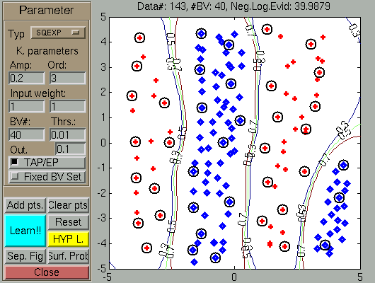
After the data addition (using the Add.Pts
and the mouse), the GP LEARNS the classification boundary, shown in the
figure with green
line. Note that since no hyperparameter learning has been
performed, the number of Basis Vectors (black circles on the figure)
is quite large.
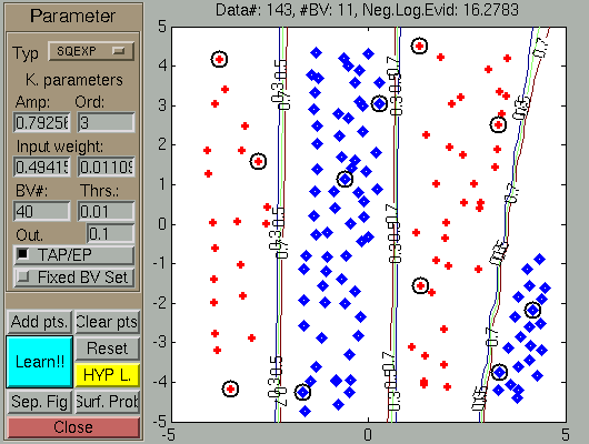
The result of a fair amount of clicking (called data generation) and
pressing the Learning
-- Hyp.opt button
pair is shown below. Observe that as a results of learning the
scaling factors changed so that the first coordinate (X-axis) became
more important than the second component, and the negative
log-evidence is much reduced.
In the next figures we show the effect of flipping the coordinates
whilst keeping the GP and the labels of the inputs.
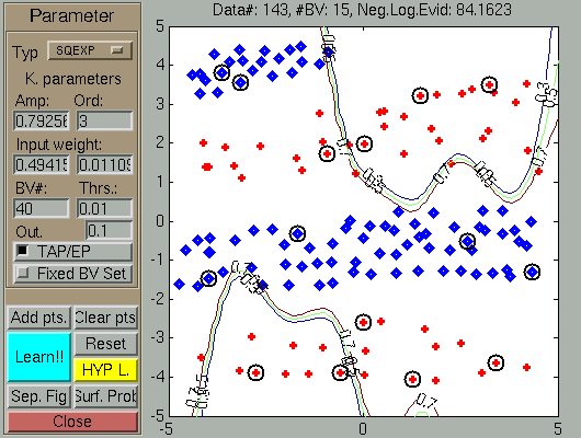
The result of changing the coordinate order. The GP is not able to learn (which is not surprising) the classification boundary.
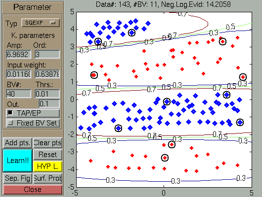
Applying several learning (Learning -- Hyp.opt) steps, the new configuration is the mirror
of the earlier final result.
Questions, comments, suggestions: contact Lehel
Csató.