Important: since it is quite technical, the text is mainly
copy-pasted from the
thesis (see
References). For more compact information you can look at the
Neural Computation article.
Online estimation of the posterior GP
The representation lemma shows that the posterior moments are
expressed as linear and bilinear combinations of the kernel functions
at the data points, allowing to tackle computationally the
posterior process.
On the other hand, the high-dimensional integrals needed for the
coefficients
q = [q1,...,
qN]T and
R = {Rij} of the posterior moments are rarely
computable analytically, the parametrisation lemma thus is not
applicable in practise and more approximations are needed.
The method used here is the online approximation to the posterior
distribution using a sequential algorithm [
55]. For this we
assume that the data is conditionally independent, thus factorising
P( |f |f ) = ) =  P(yn| fn,xn) P(yn| fn,xn)
|
(50)
|
and at each step of the algorithm we combine the likelihood of a
single new data point and the (GP) prior from the result of the
previous approximation step [
17,
58].
If

denotes the Gaussian approximation after processing
t
examples, by using Bayes rule we have the new posterior process
ppost given by
ppost(f) =
|
(51)
|
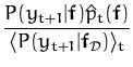
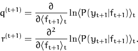
Since
ppost is no longer Gaussian, we approximate it
with the closest GP,

(see Fig.
2.2). Unlike the variational method, in this
case the ``reversed'' KL divergence
is
minimised. This is possible, because in our on-line method, the
posterior (
51) only contains the
likelihood for a single data and the corresponding non-Gaussian
integral is one-dimensional. For many relevant cases these integrals
can be performed analytically or we can use existing numerical
approximations.
Figure 2.2: Visualisation
of the online approximation of the intractable posterior
process. The resulting approximated process the from previous
iteration is used as prior for the next one.
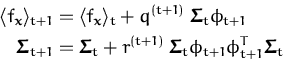
In order to compute the on-line approximations of the mean and
covariance kernel Kt we apply the Parametrisation
Lemma sequentially with a single likelihood term
P(yt|ft,xt)
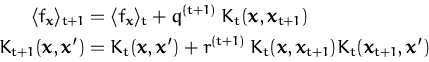
at each step. Proceeding recursively, we arrive at
|
(52)
|
where the scalars
q(t + 1) and
r(t +
1) follow directly from applying the Parametrisation
Lemma
2.3.1 with a
single data likelihood
P(
yt + 1|
xt + 1,
fxt + 1) and the process from time
t:
|
(53)
|
where ``time'' is referring to the order in which the individual
likelihood terms are included in the approximation. The averages in
(
53) are with respect to the Gaussian
process at time
t and the derivatives taken with respect to
 ft + 1
=
f (
xt + 1)
. Note again, that these averages only require a one
dimensional integration over the process at the input
xt + 1.
The online learning eqs. (
52) in the
feature space have the simple from [
55]:
|
(54)
|
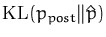
Unfolding the recursion steps in the update rules (
52) we arrive at the parametrisation for the
approximate posterior GP at time
t as a function of the initial
kernel and the likelihoods:
 fx fx
|
= |
 K0(x,xi) K0(x,xi) (i) = (i) =
 tTkx tTkx
|
(55) |
Kt(x,x ) )
|
= |
K0(x,x) +
 K0(x,xi)Ct(ij)K0(xj,x) = K0(x,x) + kxTCtkx K0(x,xi)Ct(ij)K0(xj,x) = K0(x,x) + kxTCtkx
|
(56) |
with coefficients

(
i)
and
Ct(
ij) defining the
approximation to
the posterior process, more precisely to its coefficients
q and
R from the parametrisation and equivalently in eq. (
48) using the feature space. The coefficients
given by the parametrisation lemma and those provided by the online
iteration eqs. (
55) and (
56) are equal in the Gaussian regression case
only. The approximations are given recursively as

|
(57) |
where
kt + 1 = kxt + 1
= [K0(xt +
1,x1),..., K0(xt
+ 1,xt)]T and et +
1 = [0, 0,..., 1]T is the t + 1-th unit
vector.
Observations
The
likelihood function was left unspecified. The
requirement for the online algorithm is the approximability of the
scalar coefficients
q(t+1) and
r(t+1). Several likelihood functions have this
property and the regression with Gaussian noise is the trivial example
where the integral is exact. For regression with exponential noise
the quantities are still computable. Several examples are presented
later (
Examples).
It is important that the online estimation
increases the size
of the parameters: the estimation of the posterior mean ultimately
requiring
all inputs to be stored and kernel producs to be
computed. The increasing size of parameters severely restricts the
applicability of the online estimation method to the non-parametric
GPs. The
sparse extension of the online
algorithm tackles this drawback.
Questions, comments, suggestions: contact Lehel
Csató.
![\includegraphics[]{online.eps}](thesis/img218.png)