Graph algorithms - Maximum flow of minimum cost

Maximum flow of minimum cost problem

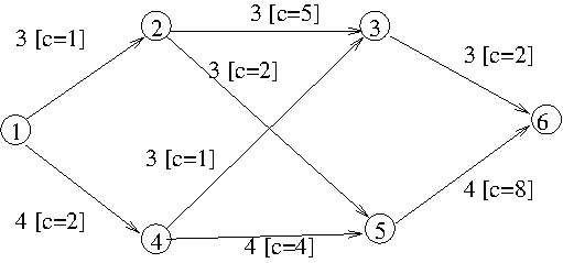
As for the maximum flow, we are given a transport network (a directed graph with capacities associated to edges, plus a source and a destination vertex). Additionaly, each edge has a cost.

In addition to the maximum flow problem, a flow also has a cost. The cost is the sum, for all edges, of the flow along the edge multiplied by the cost of the edge.

In other words, the cost of an edge is the cost of transporting each unit of flow along that edge.

The goal is to find a maximum flow and, among all possibilities to achieve it, to get one that also minimizes the cost.

Example - input graph

Solution

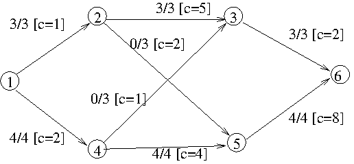
First step is to obtain a maximum flow regardless of the cost. Then we minimize the cost while keeping the value of the flow constant.

We repeat the following steps:

1. construct the residual graph
2. assign costs to edges: the cost of the original edge for the forward residual edges and minus the original cost for the backwards edges
3. find a negative cost cycle in the residual graph
4. increase the flow along the cycle (like for the augmenting paths in Ford-Fulkerson)
5. stop when no negative cost cycle exists any more

Example

Maximum flow (flow=7, cost=1*3+2*4+5*3+0*2+0*1+4*4+2*3+8*4=80):

with residual graph

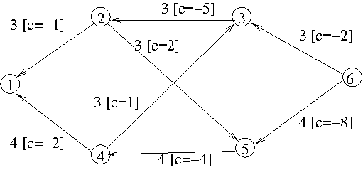
After using negative cost cycle 2, 5, 4, 3, 2 (capacity = 3, cost=-6):

with residual graph

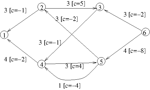
No negative cost cycle can be found. Final flow=7 of cost=80-18=62.